Social Media Popularity/Frequentation weighting for meinGrün Target Polygons
This page contains information on the process of weighting meinGrün Target shapes with additional data derived from Location Based Social Media (LBSM)
External Links:
- Code Processing (Jupyter NB - Flickr UPL HTML)
- Jupyter Notebook itself + the target shapes available on request
- Interactive maps Dresden (Flickr+Twitter+Instagram)
(in case of viewing problems, check Antivirus or Adblock)
- L0: UP Normalized, Version 5.0 (2020-03-31)
- L1: UP Normalized
- L2: UP Normalized
- L3: UP Normalized (careful: can be slow on slow hardware!)
- Interactive maps Heidelberg:
Summary:
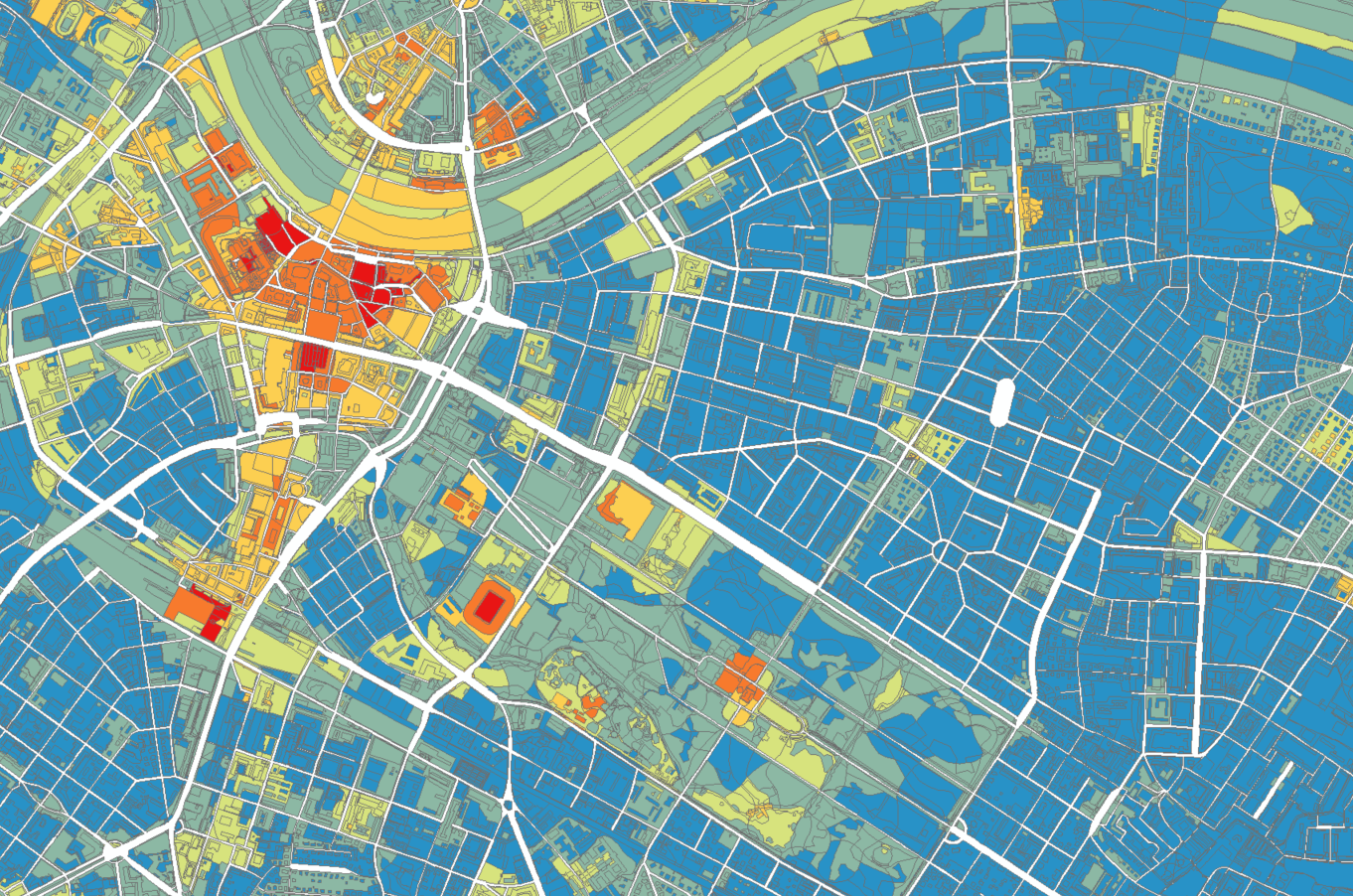
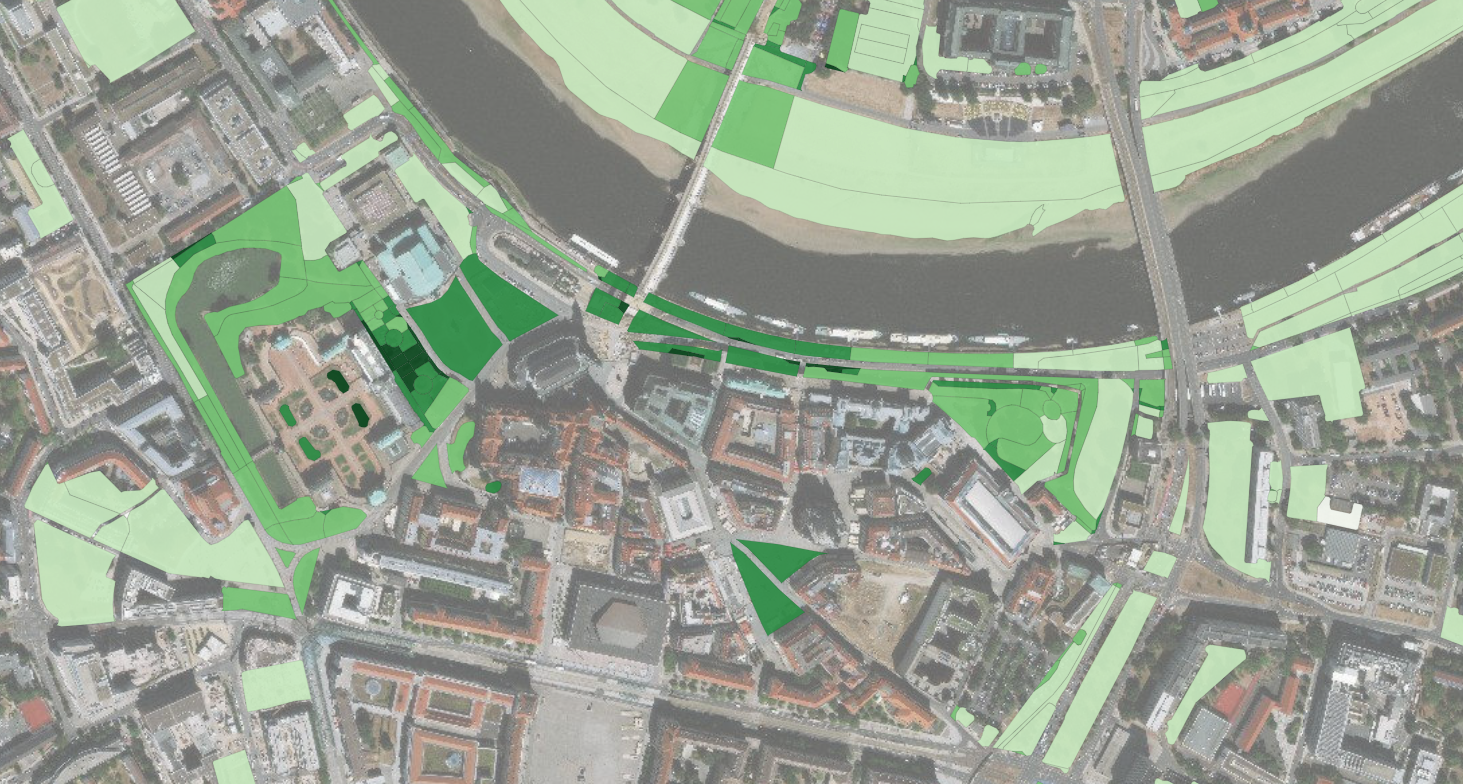
Overall, extracted tourist and public popularity per green area target appears to match subjective experiences. In Dresden, for example, the following areas are characterized with high frequentation/popularity.
- Historische Gebäude Altstadt
- Elbufer Innenstadt
- Blaues Wunde
- Fährgarten Johannstadt
- Botanischer Garten
- Palais im Großen Garten
- Hauptbahnhof
- Zoo
- Neustadt
- Elbschlösser
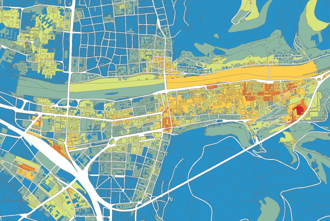
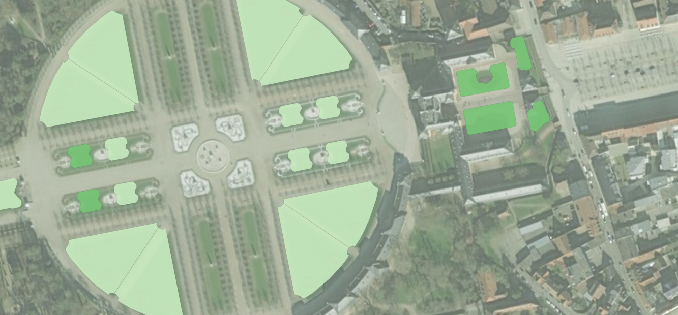
In Heidelberg, popular and highly frequented areas are equally found in the center, around Schloss Heidelberg; and around Schloss Schwetzingen.
Considerations for measuring/ processing data and common pitfalls:
the measure of density of social media posts may be referenced with “popularity” or “overall frequentation” (Beliebtheit/Frequentierung),
but there are edge cases where such references don’t work well (e.g. event locations that are only highly frequented on specific dates/times)
- it is unlikely, that any location that has many social media posts is not also frequented highly in reality
- however, there may be additional locations that are highly frequented that are not visible on Social Media
- (e.g. work-places where it is unlikely that people share photos or posts; places that are visited by particular age-groups not represented on social media etc.)
- most, but not all of these locations where many photos are shared from, do also have some aesthetic quality
- there may be locations, however, where many photos are shared from that would not be considered of high aesthetic quality
it is intended to improve these initial evaluations based on topic and time filtering , which may
- improve the measure of “popularity” or “overall frequentation”
- e.g. exclude negatively perceived topics; or information that is not relevant to the experience of green spaces (e.g. “shopping”)
- e.g. exclude temporal outliers such as event areas that are only interesting during certain times
- used to extract more detailed measurements for specific contexts
- e.g. only posts for certain activities etc.
- specific filter for extracting ‘aesthetic’ attribution of meaning
- improve the measure of “popularity” or “overall frequentation”
social media is generally biased towards tourist experiences (on average, about 70% of posts are from tourists)
- filter based on user origin may be used to produce filtered results for “locals” and “tourist”
Twitter is not fully converted into our common LBSM structure.
- We’re expecting to end the conversion of about 5TB of Twitter archive by the end of September 2019
Notwithstanding these (current) limitations, the process of relating a post to a target shape presented here will remain the same for all approaches:
- for 1st level target shapes (=L0), direct intersection (including a search radius) will be used
- for 2nd and 3rd level target shapes and raster points (L1-L3), assignment will be handled using an intermediate Kernel Density Estimation Layer, as a means to avoid outliers
Two datasets are explored here:
Filtered & Cleaned up data (referred to as
Flickr UPL in the following):
- Flickr User Post Locations (Dresden: 66.000 UPL; Heidelberg: 29.000 UPL)
- this data is of high quality, has been cleaned up and normalized based on UPL measurement
- normalization based on UPL is only for high geoaccuracy data, which is only available for a subset of the LBSM posts (most Flickr posts, some Twitter posts, no Instagram posts)
Raw data:
- Flickr + Twitter + Instagram User Posts (Dresden: about 950.000 UP; Heidelberg about 479.000 UP)
- as a means to improve the data representativity, using this source it is possible to take more data into account
- this comes with the caveat of having to deal with lower geoaccuracies and other inaccuracies
- for example, Instagram data is user-assigned to “places”, whereas a place can be everything (e.g. Instagram places exist for “Dresden”, “Germany”, “Saxony” and “Home Sweet Home”, with each of these places having only one lat-lng coordinate-pair assigned)
- we’re working on improving this extended source of information, at the moment, use information with caution
Abbreviations:
- L0-L3: These are the meinGrün target shape levels
- L0 - main targets (targets.json)
- L1 - main target parts (targetParts_Wege.json)
- L2 - mein target LC parts (targetParts_Wege_LC.json)
- L3 - main target LULC parts (targetParts_Wege_LULC.json)
- UP, UPL, UD: These are measurements for Social Media posts
- UP: Number of Photos
- UD: User days (each user is only counted once per day)
- UPL: User Post Locations (each user is only counted once per distinct location)
- A0, A1, A2, A3: These are short references to areas selected as example regions below for Heidelberg and Dresden
Data Structure Results:
Filename conventions for results: filenames follow the following pattern:
filename = {TODAY}_meingruenshapes_{TARGETSHAPE_VERSION}_{CITY_NAME.lower()}_{LEVEL}_weighted_{INTERSECT_VERSION}
where:
{TODAY}- the date of processing (yyyy-mm-dd){TARGETSHAPE_VERSION}- version of target shapes (e.g. as of 2019-09-12, v4.1 is the most recent version){CITY_NAME.lower()}- either Dresden or Heidelberg{LEVEL}- the target shape level (L0-L3, see above){INTERSECT_VERSION}- the version of the intersection code used, as of 2019-09-12, v1.1 is the most recent version
Columns:
Both shapefile and CSV include the following columns
- TARGET_ID - reference ID to input target shapes
- UP - Number of total user posts per shape
- UP_Flickr - Number of total Flickr user posts per shape
- UP_Twitter - Number of total Twitter user posts per shape
- UP_Instagram - Number of total Instagram user posts per shape
- UP_Norm - Normalized/Weighted total User posts based on Area, interpolated to 1-1000 range
- UP_Norm_Origin - Normalized/Weighted total User posts based on Area and Source of Origin, interpolated to 1-1000 range
- popularity - Natural breaks applied to UP_Norm_Origin for generating 6 bins of classes. These classes are suggestions for the overall city scale (but not meaningful when zoomed in):
- 5 : ‘very high’,
- 4 : ‘high’,
- 3 : ‘average’,
- 2 : ’low’,
- 1 : ‘very low’,
- 0 : ’no data’
Column UP_Norm_Origin is the primary meinGrün Indicator for Frequentation/Popularity
1. Data processing
1.1 Intersection Examples (L0)
The intersection, as it is implemented uses a search radius of 25m for Flickr and 50m for Instagram and Twitter surrounding meinGrün Target Shapes. The coordinates of Twitter and Instagram posts are usually less accurate, which is why a larger search radius is used for these two. The Graphic below illustrates a Target Shape (blue) in the Park of Schwetzingen Palace, the two Search_Radius distances (yellow and red dashed lines) and the Social Media posts (yellow) that were preselected using a bounding box. All Twitter and Instagram posts inside the orange dashed lines will be counted. For Flickr, every post inside the red dashed line is counted (25m).
.png)
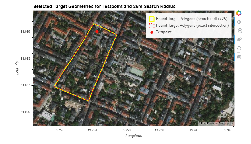
The images below illustrate a range of other test cases, with short discussions, for intersecting post with target shapes.
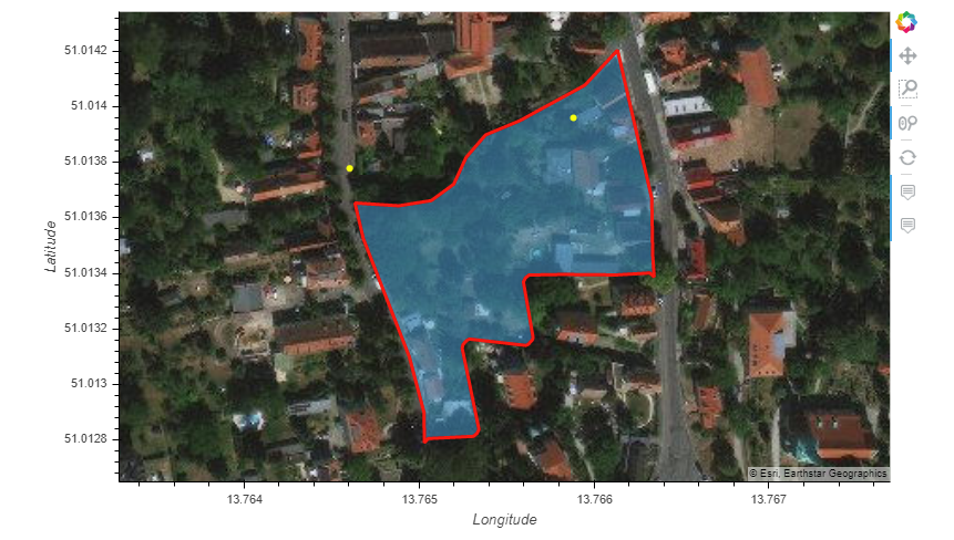
The following map shows a meinGrün Target Shape and two social media posts (yellow dots), which will be counted for the given shape.
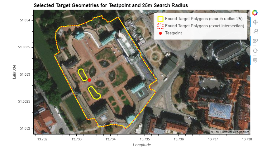
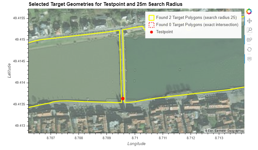
The question whether it is better to use exact intersection or intersection based on a search radius is not clear cut for all examples.
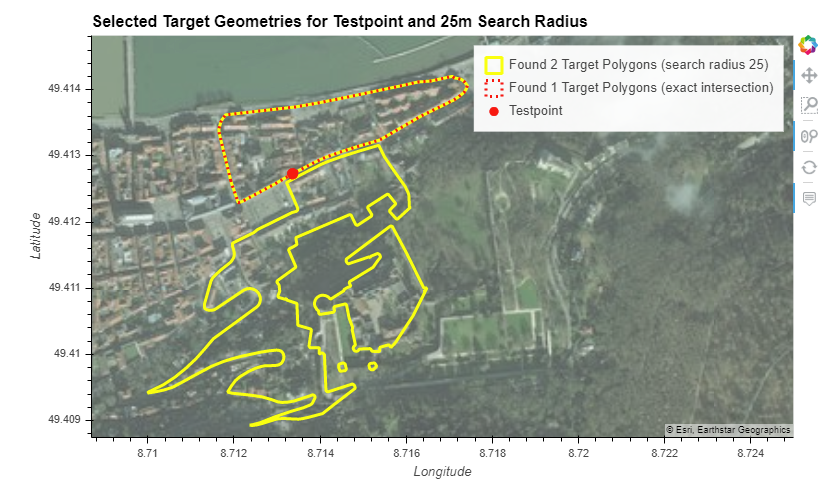
In the following case, one could argue that both solutions work. We decided for search radius in this case, because there clearly is a relation between the post and the two flower beds in the Zwinger.
Using a search radius of 25 m means all 3 target shapes will be incremented by 1 User Post Location (UPL), the assignment in this case therefore bears some ambiguity.
Other cases are more clear-cut:
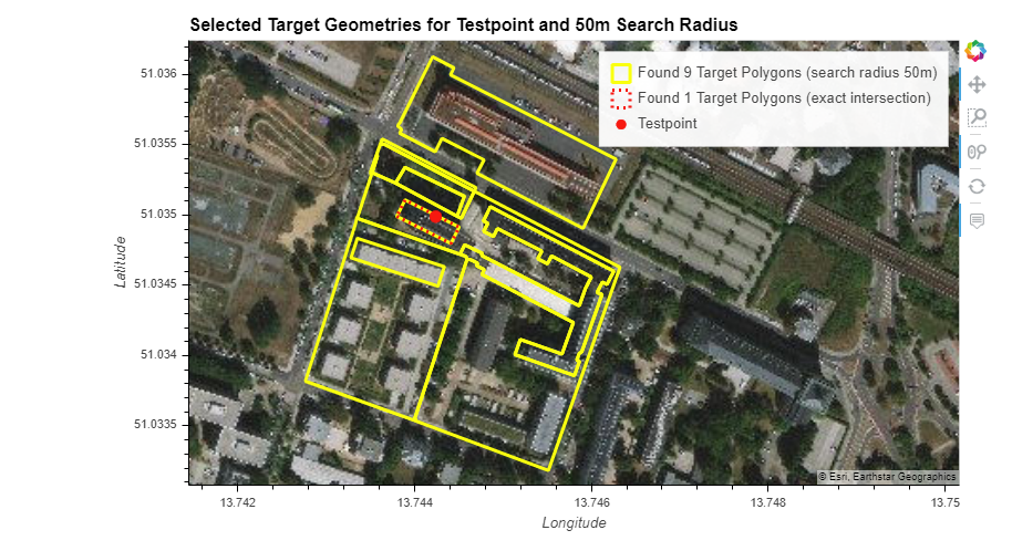
Some issues arise, when there’re complex and large target polygons: (at this level of target shapes, there is not much that can be done - we’ll illustrate the fine grained target shapes later)
- note that this specific example has been resolved by subdividing target shapes of the Großer Garten
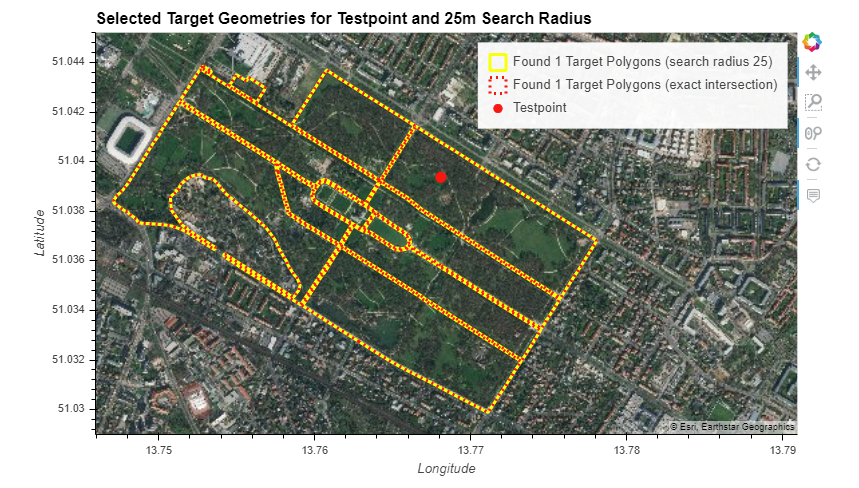
In the following case, using a search radius is clearly preferred, since the post location falls in the middle of the Großer Garten target shapes and wouldn’t be counted on exact intersection:
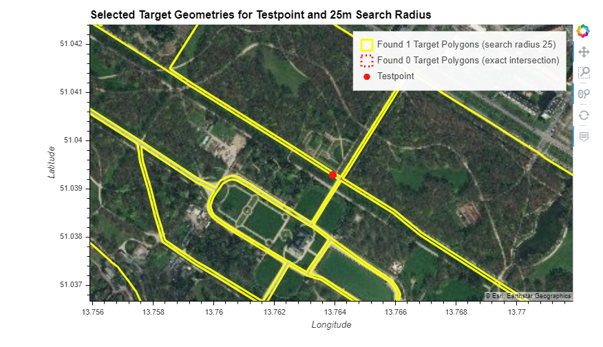
This example is again not clear-cut. However, if someone took a photo from these stairs along the Elbe river terrace, one may argue that the photo is not of the stairs but of the perceived river shore lying in front. Therefore it makes sense to increment both target shapes.
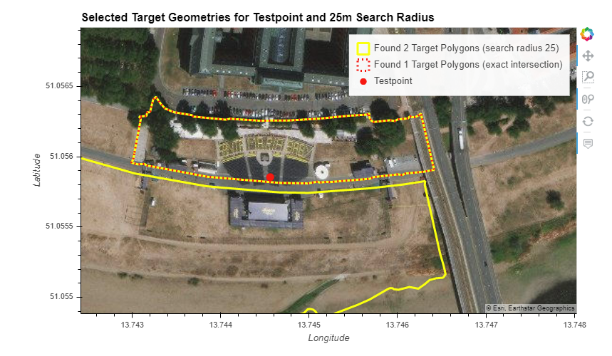
These are two other edge cases, where accurate assignment to either one of the two shapes seems difficult:
Another example for L2 Target Layer and 50m Search Radius (Instagram/Twitter):
1.2 Normalizing and Weighting data
There are different measurements that provide different insights into social media patterns. What is counted:
- User Posts (UP): A User Post is the simplest measurement, but it includes also many biases that affect accuracy of results: - some users and cultural groups always take and share more photos than others, these groups will be over-represented in User Post Measure - manually geolocated social media posts with low geoaccuracy may distort results, for example, if a user drops all 200 (e.g.) posts of an album on a single coordinate, the final map may show a misleading peak of user posts in this area - some topics on social media are typically always represented with more photos than other topics, such as tourist landmarks or places where people and groups frequently meet, these places will be over-represented in UP measurement
- User Days (UD): Each user will be counted once per day for each location or meinGrün Target shape. The advantage of using User Days as measurement is that locals will have a higher effect on results than tourists, because locals usually visit their favorite places consecutively/frequently on multiple days.
- User Post Location (UPL): UPL count users at each location only once, whereas location can be defined as a tuple of coordinates (lat lng) or other bases such as a “meinGrün target shape”. This will specifically reduce the affect of low geoaccuracy information in georeferenced social media posts. For example, when users on Flickr manually georeference their content, many will simply drop all posts of a photo album on a single coordinate. Counting each photo of these albums separately will introduce inaccuracies and biases in final results. A UPL simply has all posts of a single user at a single coordinate merged, e.g. a reduced list of terms, tags and emoji based on global occurrence (i.e. no duplicates). UPL have the caveat that amount of available data is heavily reduced, therefore UPL are usually not suited for large scale evaluations
We calculate these measurements per meinGrün target shape. The resulting table looks similar to this one:
| TARGET_ID | UP | UD | UPL | UP_Instagram | UP_Flickr | UP_Twitter | |
|---|---|---|---|---|---|---|---|
| 24384 | dd_EBK-TSP-OSM_30690 | 35621 | 28946 | 24810 | 35054 | 567 | 0 |
| 1758 | dd_EBK-TSP-OSM_33708 | 8011 | 6375 | 5965 | 6983 | 1028 | 0 |
| 22702 | dd_EBK-TSP-OSM_20688 | 37789 | 31835 | 28202 | 34809 | 2967 | 13 |
| 8449 | dd_EBK-TSP-OSM_26112 | 3457 | 2375 | 1895 | 3025 | 432 | 0 |
| 16013 | dd_EBK-TSP-OSM_24972 | 3368 | 2368 | 1879 | 3025 | 343 | 0 |
It becomes obvious that Instagram dominates results. We need to normalize measurements:
- using the target shape’s area (otherwise, larger shapes would dominate results)
- using the overall distribution of service origin
- For Dresden, the distribution is:
- Instagram posts have a percentage of: 81.34%
- Flickr posts have a percentage of: 18.49%
- Twitter posts have a percentage of: 0.17%
- For Heidelberg, the distribution is:
- Instagram posts have a percentage of: 70.52%
- Flickr posts have a percentage of: 29.20%
- Twitter posts have a percentage of: 0.28%
- each data source should have an equal base effect on final results
- For Dresden, the distribution is:
- finally, we manually reduce Twitter & Instagram influence, since these source have overall lower geoaccuracies. Twitter, in addition, can introduce sampling effects due to low data density.
- therefore, after global origin normalization, we added the following modifiers:
- 40% Influence by Instagram (reduced because Instagram has low geoaccuracy)
- 50% Influence by Flickr (increased because Flickr featurss highest geoaccuracy)
- 10% Influence by Twitter (reduced because twitter features sampling noise)
- therefore, after global origin normalization, we added the following modifiers:
Examples Normalization
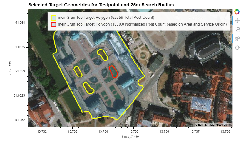
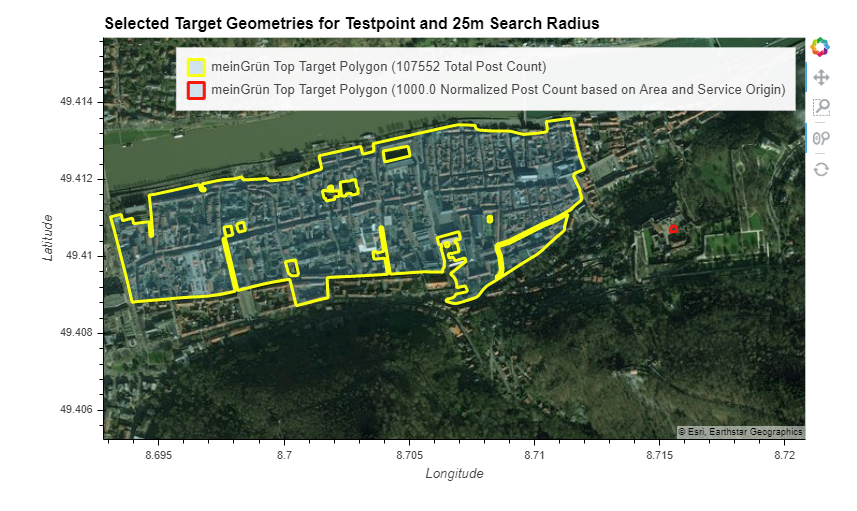
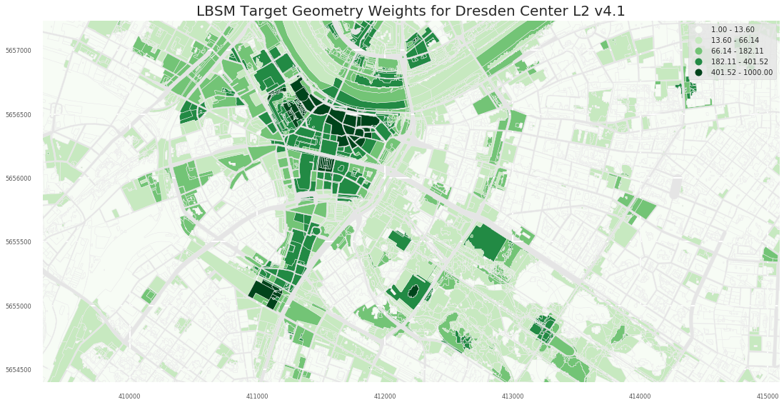
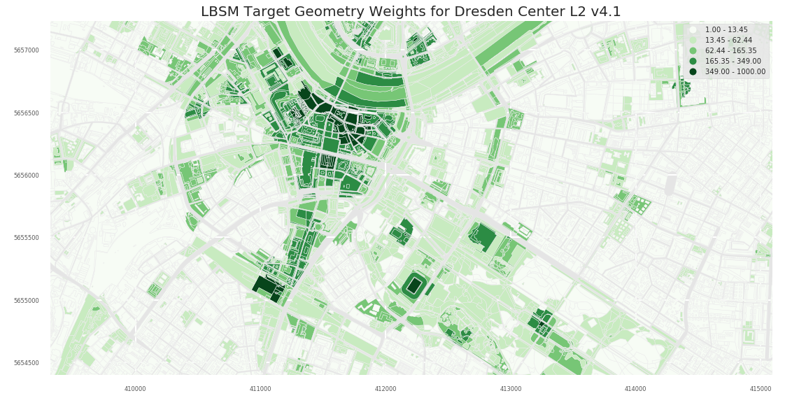
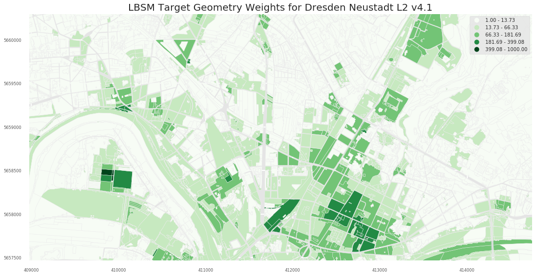
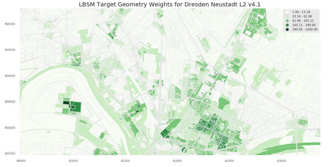
The following graphics shows the top target shape for Dresden, based on Post Count (UP)
- yellow: top target polygon without area normalization
- red: top target polygon with area normalization
The same for the L2 Layer shows that assignment remain stable across different granularities:
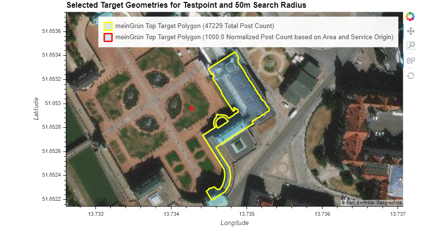
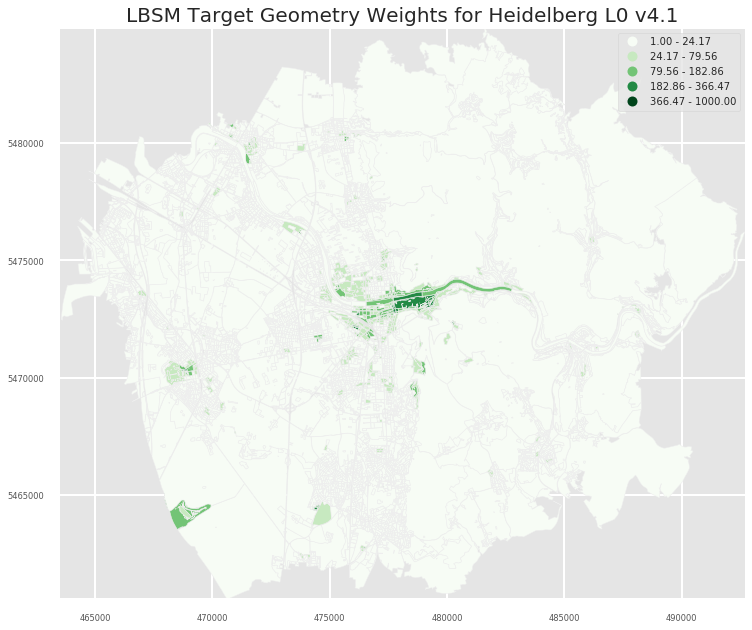
In Heidelberg, the difference is more easily visible:
Final values are stretched to a 1 to 1000 range. This range of values is assigned to a measurement of “popularity”, based on natural breaks algorithm:
- very high
- high
- average
- low
- very low
- no data
Example Results
Lets compare some of these results.
Interactive maps:
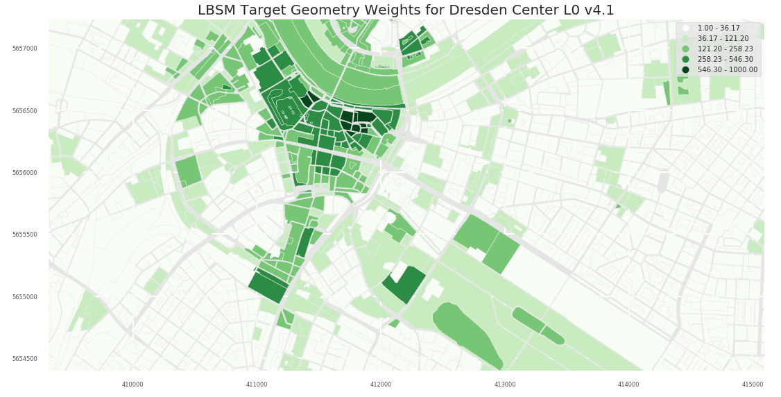
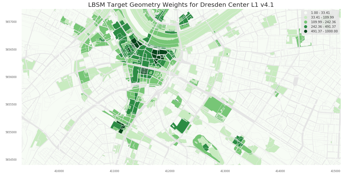
2. Results
2.1 Dresden
2.1.1 A1
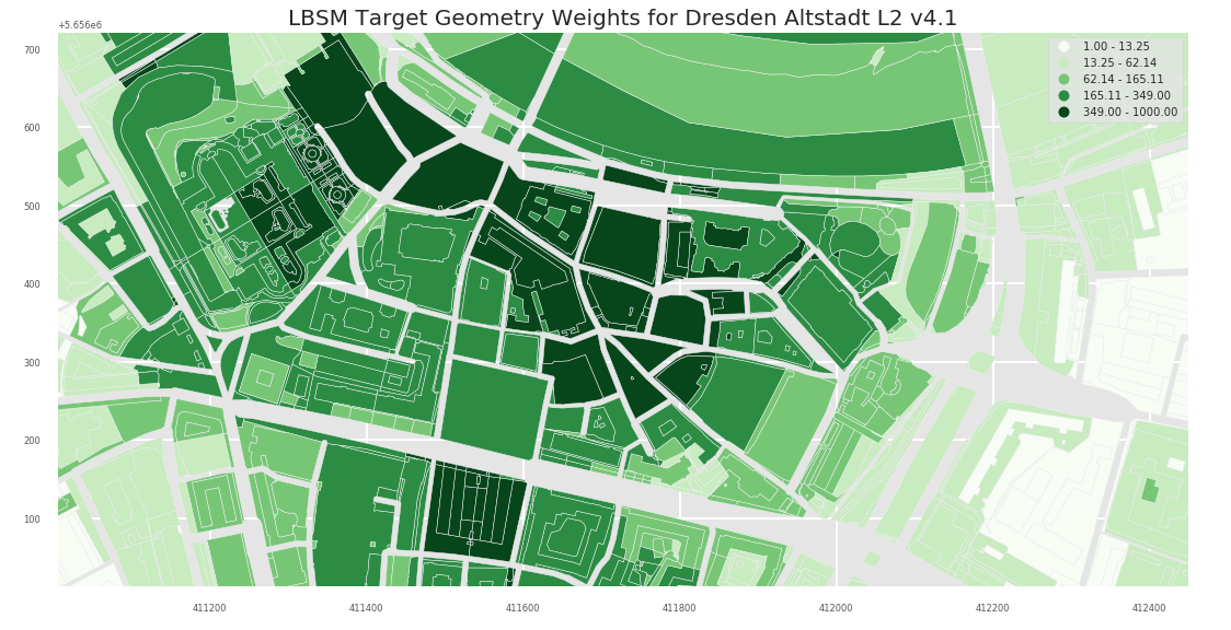
- L0
- L1
- L2
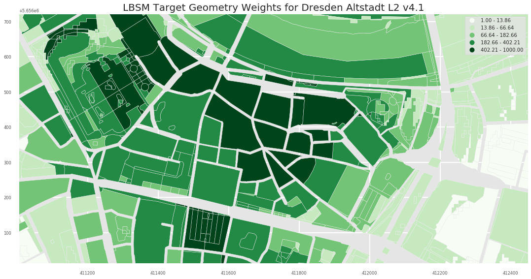
- L3
2.1.2 A2
- L0
- L1
- L2
- L3
2.1.3 A3
- L0
- L1
- L2
- L3
ArcMap Natural Breaks (L3):
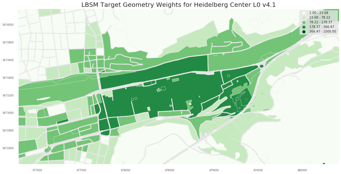
2.2 Heidelberg
2.2.1 A0
- L0
- L1
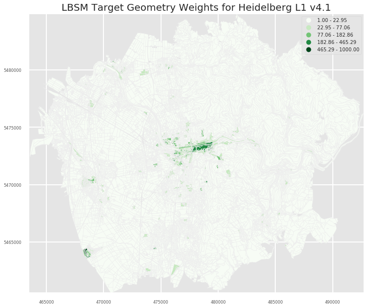
- L2
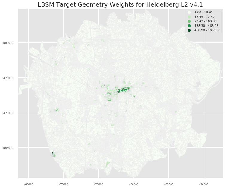
- L3
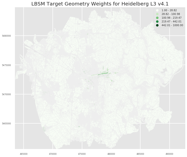
2.2.2 A1
- L0
- L1
- L2
- L3
2.3 Selected areas
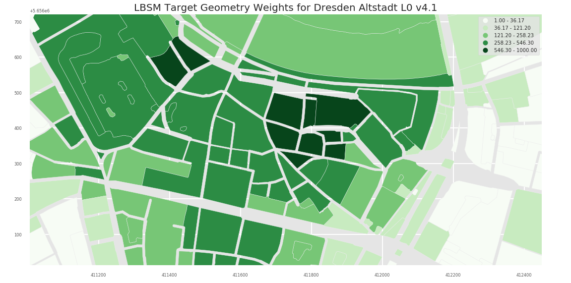
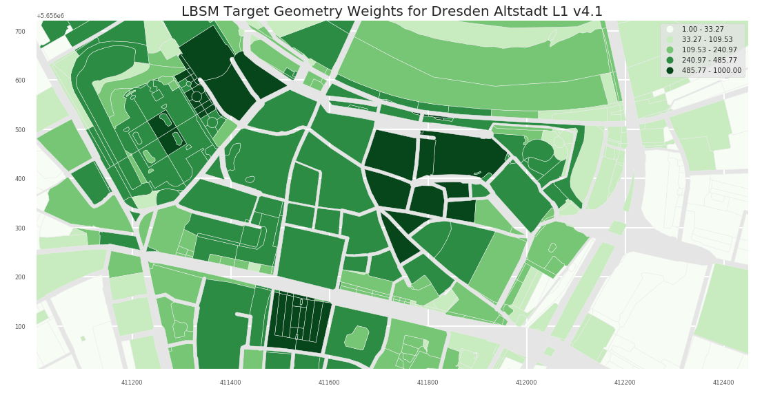
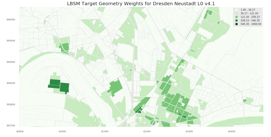
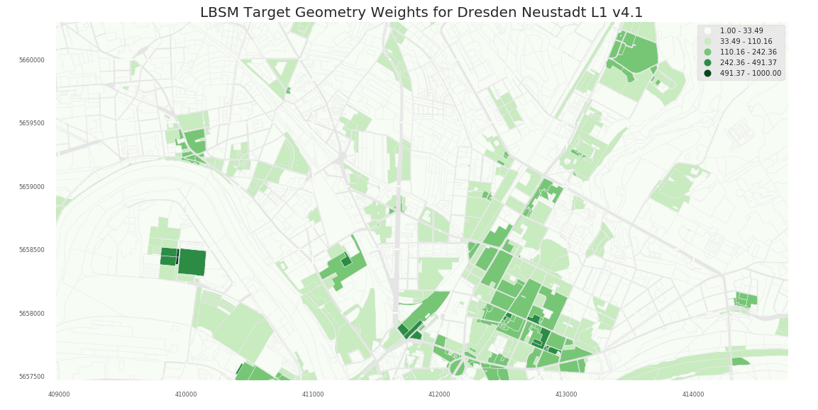
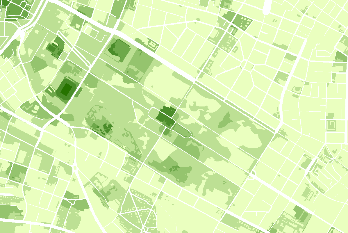
L1 Level provides a more fine grained picture:
Pillnitz
Dresden Altstadt
Schloss Heidelberg
Schloss und Schlossgarten Schwetzingen
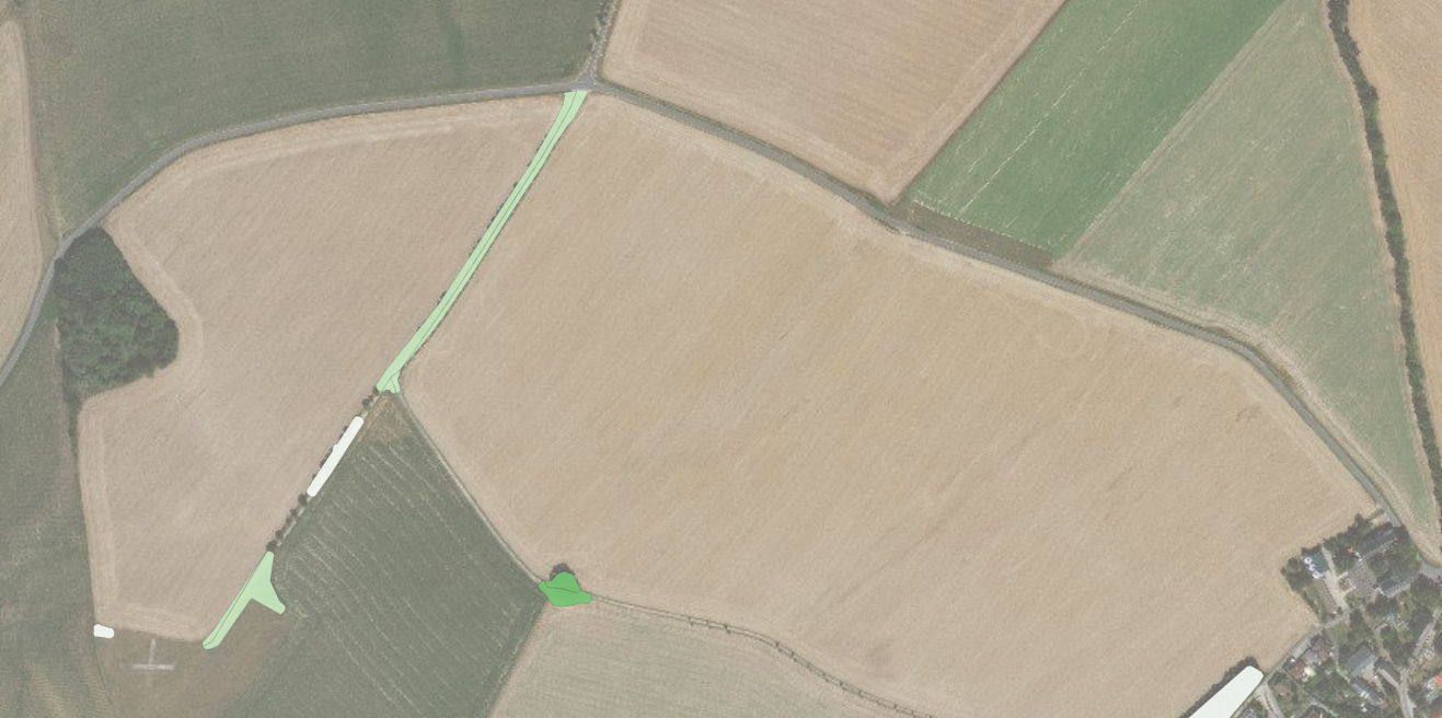
.. but also remote places, such as the Babisnauer Pappel, show I higher popularity than surrounding areas:
3. Datasets
Exported datasets include:
- a CSV with column TARGET_ID (meinGrün Target-geometry ref) and LBSM columns
- UP,UP_Flickr,UP_Twitter,UP_Instagram,UD,UPL,UP_Norm,UP_Norm_Origin,popularity
- a Shapefile with the same columns
The two recommended measurement:
- popularity: labeled based on natural breaks and UP_Norm_Origin - recommended classes for overall city level
- UP_Norm_Origin: 1 to 1000 interpolated range weights for Social Media - apply individual classes
The exported datasets are available on request.