I just finished a data processing task where I encountered several challenges while processing a large geosocial media dataset (~60 million posts) to aggregate activity at the German postal code (PLZ) level.

The broader context for this work is a project aiming to integrate insights from the Socio-Economic Panel (SOEP) Data from DIW Berlin with patterns derived from geosocial media. SOEP provides rich panel data typically collected on a 5-year basis, while geosocial media offers a more continuous, albeit different, lens on societal activity. To effectively complement these datasets and to identify gaps or differences, we plan to conduct on-site questionnaires or mail surveys. For such survey logistics, PLZ areas are the most practical geographical unit due to their direct relevance in mail and address management.

Intersecting and Aggregating Geosocial Data with PLZ Geometries

The initial task was to intersect approximately 60 million geosocial media posts (from platforms like Instagram, Flickr, Twitter, iNaturalist) with around 9,000 PLZ area geometries for Germany. To maintain user privacy while still getting activity counts, we use HyperLogLog (HLL) for estimating unique user and post counts per PLZ. The raw post data resides in a PostgreSQL/PostGIS database, and the plan was to use a materialized view (mviews.all_posts_de) representing all posts in Germany, and join this with a table of PLZ geometries (mviews.plz_intersect).

The core aggregation query looks something like this (see full notebook):

CREATE MATERIALIZED VIEW mviews.plz_social_de AS
    SELECT
        plz.plz,
        plz.geom,
        hll_add_agg(hll_hash_text(s.user_guid)) as user_hll,
        hll_add_agg(hll_hash_text(s.post_guid)) as post_hll
    FROM mviews.plz_intersect AS plz
    JOIN mviews.all_posts_de AS s -- FDW or local materialized view
    ON plz.geom && s.post_latlng AND ST_Intersects(plz.geom, s.post_latlng)
    GROUP BY plz.plz, plz.geom;

Initially, this query ran for 24 hours before I realised that something was wrong. I realised that Postgres materialised views do not inherit their parent table’s indexes. This meant that Postgres was performing 450 billion geometry comparisons, equating to 9000 × 50,000,000.

The lack of spatial indexes on either the mviews.plz_intersect table (containing ~9,000 PLZ polygons) or the mviews.all_posts_de materialized view (containing ~50 million post locations) meant PostGIS was performing a massive number of raw geometry comparisons.

The fix was to explicitly create spatial GIST indexes on both tables involved in the spatial join:

1. Index for the PLZ geometries table:

   CREATE INDEX idx_plz_intersect_geom ON mviews.plz_intersect USING GIST (geom);
   ANALYZE mviews.plz_intersect;
   

2. Index for the materialized view containing all post locations:

   CREATE INDEX IF NOT EXISTS idx_mv_all_posts_de_post_latlng_gist
   ON mviews.all_posts_de USING GIST (post_latlng);
   ANALYZE mviews.all_posts_de;
   

Additionally, for Foreign Data Wrappers (FDW), ensuring use_remote_estimate is enabled can help the planner:

ALTER SERVER lbsnraw OPTIONS (SET use_remote_estimate 'on');
ALTER FOREIGN TABLE mviews.all_posts_de OPTIONS (ADD use_remote_estimate 'true');

After implementing these indexes, the query execution time for creating mviews.plz_social_de dropped dramatically from “days” to approximately 2 hours. The resulting table provides HLL objects for user and post counts per PLZ, which can then be queried for cardinality estimates.

Visualization and Cluster Analysis of PLZ-Level Geosocial Patterns

With the aggregated data (user counts and post counts per PLZ) exported to a CSV, the second phase involved visualization and exploratory spatial data analysis using Python (GeoPandas, Matplotlib, Seaborn, HDBSCAN).

The key steps in this notebook include:

1. Loading Data: Reading the PLZ shapefiles and merging them with the geosocial counts.

2. Basic Choropleth Mapping: Visualizing raw user counts using different classification schemes (e.g., Quantiles, Natural Breaks).

3. Ratio Analysis:

   • Calculating active geosocial users per capita (user_pop_ratio).
   • Calculating the inverse: population per active user (pop_user_ratio) to highlight areas with high population but relatively low geosocial activity.
   • Applying log transformations (np.log1p) to handle skewed distributions of these ratios for better visualization.

4. Area Normalization: To account for the Modifiable Areal Unit Problem (MAUP) where large PLZ areas might distort simple ratios, densities were calculated (population density, user density) and a density_ratio (population density / user density) was derived.

5. Filtering for Robustness: Selecting PLZs for deeper analysis by applying thresholds (e.g., minimum 5,000 residents, minimum 5,000 users, maximum PLZ area of 50 km²) to focus on statistically relevant and comparable areas.

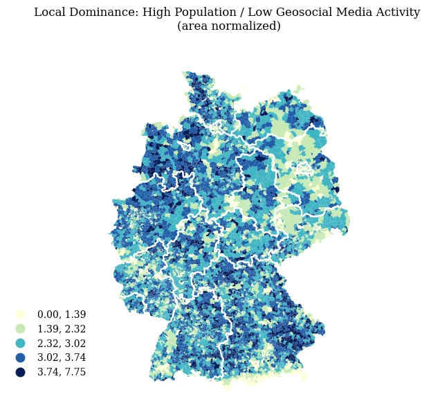   Fig 1: Visualization of selected PLZ areas based on geosocial media and population density ratios.

6. Geographic Clustering (HDBSCAN):

   • The filtered subset of PLZs (those with high population relative to geosocial activity, meeting size/count criteria) was then subjected to geographic clustering using HDBSCAN.
   • Centroids of the selected PLZs were used as input, with the Haversine metric for distance calculation. min_cluster_size was a key parameter tuned to identify meaningful spatial groupings.

7. Expanding Clusters to Contiguous Areas:

   • To create more practical, contiguous regions from the (potentially scattered) PLZs within each HDBSCAN cluster, an approach involving convex hulls and buffering was implemented:
     1. For each HDBSCAN cluster, the unary_union of its member PLZ geometries was taken.
     2. A convex_hull was generated around this union.
     3. This hull was then buffered (e.g., by 1000 meters).
     4. All PLZs from the complete German PLZ dataset that intersected these buffered hulls were selected and assigned the respective expanded cluster ID.
     5. These selected PLZs were then dissolved by their new expanded_cluster_id to form the final, more contiguous, expanded cluster areas.

This process is used for the identification and delineation of broader regions exhibiting specific socio-geospatial characteristics. The resulting GeoDataFrames (selected PLZs, HDBSCAN clusters, and expanded cluster areas) are exported to GeoPackage, Shapefile, and CSV formats.

The full notebooks can be found at 06_plz_intersection.html and 07_plz_visualization.html.