Part 4: Topic Classification of Social Media 
Workshop: Social Media, Data Science, & Cartograpy
Alexander Dunkel, Madalina Gugulica
This is the fourth notebook in a series of four notebooks:
- Introduction to Social Media data, jupyter and python spatial visualizations
- Introduction to privacy issues with Social Media data and possible solutions for cartographers
- Specific visualization techniques example: TagMaps clustering
- Specific data analysis: Topic Classification
Open these notebooks through the file explorer on the left side.
The task in this notebook is very similar to the one presented in the previous notebook Part3 - Tag Maps Clustering and Topic Heat Maps, namely to explore the latent topics from LBSM data and visualize the textual information and its spatial distribution for a given topic. The emphasis in this notebook lies, however, on data exploration and analysis rather than on data visualization and focuses on a method of classifying social media posts based on the textual metadata.
For this notebook, we use a another environment that must be linked first.
!cd .. && sh activate_topic_env.sh
Important:
- In this notebook we will be working with RAW Instagram data since the method approached hasn't been applied on the HLL datastructure
- Please:
- Do not share the original data
- Remove original data after the workshop
Introduction: Social Media & Topic-based text classification
The content social media users share on different platforms is extremely diverse encompassing a very wide range of topics including valuable information related to the way people perceive, relate to and use different environments. In order to harness these large volumes of data, specific tools and techniques to organize, search and understand these vast quantities of information are needed.</br>
Text classification is a Natural Language Processing task that aims at mapping documents (in our case social media posts) into a set of predefined categories. Supervised machine learning classifiers have shown great success in performing these tasks. Nevertheless, they require large volumes of labeled data for training, which are generally not available for social media data and can be very time-consuming and expensive to obtain.</br>
This notebook introduces a practical and unsupervised approach (which requires no labeled data) to thematically classify social media posts into specific categories (topics) simply described by a label. The underlying assumption of this approach is that Word Embeddings can be used to classify documents when no labeled training data is available. </br>
The method is based on the comparison of the textual semantic similarity between the most relevant words in each social media post and a list of keywords for each targeted category reflecting its semantics field (in linguistics, a semantic field is a set of words grouped by their meaning, that refers to a specific subject). The strenght of this approach is represented by its simplicity, however, its success depends on a good definition for each topic reflected in the list of keywords.</br>
Methodology
How do we make machines understand text data? It is generally known that machines are experts when dealing and working with numerical data but their performance decreases if they are fed raw text data.
The idea is to create numerical representation of words that capture their meanings, semantic relationships and the different contexts they are used in. For the coversion of raw text into numbers, there are a few options out there. The simplest methodology when dealing with text is to create a word frequency matrix that simply counts the occurrence of each word ( bag-of-words). An enhance version of this method is to estimate the log scaled frequency of each word considering its occurrence in all documents (tf-idf). Nevertheless, these methods capture solely frequencies of words and no contextual information or high level semantics of text.
A recent advance on the field of Natural Language Processing proposed the use of word embeddings for the numerical representation of text.
Word Embeddings
Word embeddings are a type of word representation that allows words with similar meaning to have similar representations. Behind the approach of learning these representation lies the “distributional hypothesis” by Zellig Harris, a linguistic theory that could be summarized as: words that have similar context will have similar meanings.
Word2Vec embedding approach Word2Vec is one of the most popular word embedding models and it was introduced in two papers between September and October 2013, by a team of researchers at Google and is considered the state of the art. Word2Vec approach uses deep learning and neural networks-based techniques to convert words into corresponding vectors in such a way that the semantically similar vectors are close to each other in N-dimensional vector space, where N refers to the dimensions of the vector. As words that have similar neighbouring words are likely semantically similar, this means that the word2vec approach is very good at capturing semantic relationships.
Word2Vec's ability to capture and maintain semantic relationships is reflected by a famous classic example where if you have a vector for the word "King" and you remove the vector represented by the word "Man" from the "King" and add "Woman" to it, you get a vector which is close to the "Queen" vector. This relation is commonly represented as: King - Man + Woman = Queen.
Word2Vec can be used to find out the relations between words in a dataset, compute the similarity between them, or use the vector representation of those words as input for applications such as text classification.
For more information on Word Embeddings this could be a starting reading material: https://ruder.io/word-embeddings-1/index.htmlThe method adopted computes the semantic similarity between different words or group of words and determines which words are semantically related to each other and belong to the same semantic field. Furthermore, computing the distance in the vector space (cosine distance) between the centroid of the word vectors that belong to a certain topic (semantic field) and the centroid of the word vectors that compose a social media posts will allow us to verify if the textual metadata associated with the posts is related to a specific category (Binary Classification).
In this notebook we will implement the Word2Vec word embedding technique used for creating word vectors with Python's Gensim library. </br>
1. Preparations
Load Dependencies
import pandas as pd
import pickle
import scipy
import numpy as np
import matplotlib.pyplot as plt
import warnings
warnings.filterwarnings('ignore')
from IPython.display import clear_output, Markdown, display
We're creating several output graphics and temporary files.
These will be stored in the subfolder notebooks/out/.
from pathlib import Path
OUTPUT = Path.cwd() / "out"
OUTPUT.mkdir(exist_ok=True)
1.1. Load the pre-trained Word2Vec model and the idfscores dictionary
The model was trained on a corpus, that has been previously prepared by filtering, cleaning and normnalizing over 1.5 M Instagram, Flickr and Twitter posts geolocated within Dresden and Heidelberg.
Parameters were chosen according to the semantic similarity performance results reported in *Efficient Estimation of Word Representations in Vector Space* - T. Mikolov et al.(2013)
- size (vector size): 300
- alpha (initial learning rate) : 0.025
- window: 5
- min_count: 5
- min_alpha: 0.0001 Learning rate will linearly drop to min_alpha as training progresses
- sg: 1 (SkipGram architecture - predicting context words based on current one)
- negative (negative samples): 5 If > 0, negative sampling will be used, the int for negative specifies how many “noise words” should be drawn (usually between 5-20). If set to 0, no negative sampling is used.
- ns_exponent = 0.75 The exponent used to shape the negative sampling distribution. A value of 1.0 samples exactly in proportion to the frequencies, 0.0 samples all words equally, while a negative value samples low-frequency words more than high-frequency words. The popular default value of 0.75 was chosen by the original Word2Vec paper.
- iter : 15 Number of iterations (epochs) over the corpus.
%load_ext autoreload
%autoreload 2
Prepare paths..
import sys

INPUT = Path.cwd() / "input"

module_path = str(Path.cwd().parents[0] / "py")
if module_path not in sys.path:
    sys.path.append(module_path)
from modules import tools
source = "topic_data.zip"
Download sample data. This may take some time.
%%time
sample_url = tools.get_sample_url()
zip_uri = f'{sample_url}/download?path=%2F&files='
tools.get_zip_extract(
    uri=zip_uri,
    filename=source,
    output_path=INPUT,
    write_intermediate=True)
load the pretrained word2vec model usign gensim's Word2Vec
from gensim import utils
from gensim.models import Word2Vec
model_w2v = Word2Vec.load(
    str(INPUT / "word2vec.model"))
For the creation of the post_embedding we will need idf-score weights, which were prepared beforehand and stored in the input folder as a serialized (pickled) dictionary
#idf-scores dictionary deserialization
with open(INPUT / 'idf_scores_dict.pkl', 'rb') as handle:
    idf_scores_dict = pickle.load(handle)
1.2. Define the functions that will help compute the average topic and post vectors
Functions to compute the average topic and post vectors
def avg_topic_vector(lang_model, tokens_list):
    # remove out-of-vocabulary words
    tokens = []
    for token in tokens_list:
        if token in lang_model.wv.vocab:
            tokens.append(token)
    return np.average(lang_model[tokens], axis=0)

def avg_post_vector(lang_model, tokens_list,idf):
    # remove out-of-vocabulary words
    tokens = []
    weights = []
    for token in tokens_list:
        if token in lang_model.wv.vocab:
            tokens.append(token)
            tf = tokens_list.count(token)
            tfidf= tf*idf[token]
            weights.append(tfidf)
    return np.average(lang_model[tokens], weights =weights, axis=0)


def has_vector_representation(lang_model, upl):
    """check if at least one word of the document is in the
    word2vec dictionary"""
    n= len([w for w in upl if w in lang_model.wv.vocab])
    if n>0:
        return True
    else:
        return False
2. Load Preprocessed Data
The textual content of social media data has a low degree of formal semantic and syntactic accuracy. In order to provide only significant information for the text classification task to be performed, the text (posttitle, post body and tags) needed to be preprocessed according to the following actions:
- lowercasing
- extract hashtags and individual words (tokenization)
- remove mentions (@username)
- remove punctuation
- remove the URLs (http:\ as well as www.)
- remove html tags (<>)
- remove digits
- identify and select only English and German posts
- remove stopwords (commonly used words such as “the”, “a”, “an”, “in”, etc.)
filename = "DD_Neustadt_NormalizedInstagramPosts.pickle"
df = pd.read_pickle(INPUT / filename)
print(len(df))
df.head()
3. Topic-Based Classification of Social Media Posts
Workflow
The classification of the social media posts is based on the calculation of the similarity score (cosine similarity) between a topic embedding & the post embeddings and follows the workflow exposed below:
for each label (topic) a list of relevant keywords is defined and enhanced by seeking further semantically similar words through the identification of the most similar word vectors (which are closely located in the vector space)
a topic embedding will be created by averaging all the vectors representing the keywords in the list previously defined
the vector represention of each social media post is created by averaging the weighted word embeddings of all words and the weight of a word is given by its tf-idf score.
TF-IDF
Tf-idf, short for term frequency - inverse document frequency, is a statistical measure that evaluates how relevant a word is to a document in a collection of documents. This is done by multiplying two metrics: how many times a word appears in a document, and the inverse document frequency of the word across a set of documents. The tf-idf score is: - highest when a occurs many times within a small number of documents (thus lending high discriminating power to those documents); - lower when the term occurs fewer times in a document, or occurs in many documents (thus offering a less pronounced relevance signal); - lowest when the term occurs in virtually all documents.- the classification will follow after the calculation of a similarity score between each pair of post vector - topic vector using cosine distance and an empirically identified similarity threshold (70%) is considered decisive
Use your own input by changing the keywords in the list below and explore other topics that you are interested in. Try to input more than one keyword to "define" the topic as specifically as possible.
topic_list = ['event','music','festival','concert']
gensim.models.Word2Vec.most_similar finds the top-N most similar words. Positive words contribute positively towards the similarity, negative words negatively.This method computes cosine similarity between a simple mean of the projection weight vectors of the given words and the vectors for each word in the model. The method corresponds to the word-analogy and distance scripts in the original word2vec implementation.
Apply the same method to find semantically similar words for your input!
enhanced_list = []
for keyword in topic_list:
    similar_words = model_w2v.wv.most_similar(
        positive = [keyword], topn = 50)
    enhanced_list += ([w[0] for w in similar_words])
some words might repeat, therefore we will save the list as a set of unique strings
topic_list = topic_list + enhanced_list
topic_list = set(topic_list)
To create the topic embedding call the previously defined avg_topic_vector function.
topic_embedding = avg_topic_vector(model_w2v,topic_list)
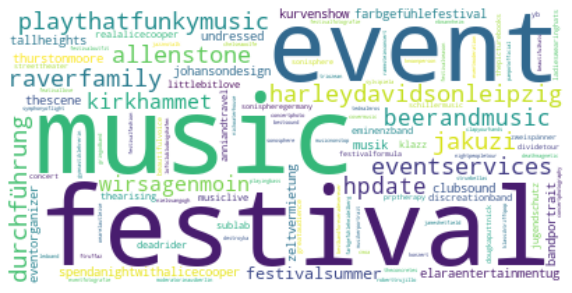
WordCloud representing the topic selected
To visualize the enhanced list of keywords representative for the chosen topic and used for the calculation of the topic embedding, we use the WordCloud library.
Note: Some of the tags identified might refer to the city of Heidelberg since the word2vec model was trained on social media posts that were published within both Dresden and Heidelberg.
import matplotlib.pyplot as plt
from wordcloud import WordCloud
words = ' '.join(topic_list)
wordcloud = WordCloud(background_color="white").generate(words)
# Display the generated image:
plt.figure(figsize = (10,10))
plt.imshow(wordcloud, interpolation='bilinear')
plt.axis("off")
plt.show()

We will add 2 new columns to the dataframe "classification" and "cos_dist" to save the classified Instagram posts as a dataframe that will be pickled and store in the output folder. Accordingly, the "classification" column will be populated with the ones (if the post_text reflects the topic selected and the calculated cosine distance is smaller than 0.3) and zeros (if the calculated cosine distance is larger than 0.3). We store the cosine distance values in the "cos_dist" column for further inspections.
%%time
df = df.reindex(df.columns.tolist() + ['classification','cos_dist'], axis=1)
x = 0
total_records = len(df)
for index, row in df.iterrows():
    x+=1
    msg_text = (
        f'Processed records: {x} ({x/(total_records/100):.2f}%). ')
    if x % 100 == 0:
        clear_output(wait=True)
        print(msg_text)

    text = row['post_text'].split(' ')

    if has_vector_representation(model_w2v, text) == True:
        #create the post embedding
        post_embedding = avg_post_vector(model_w2v, text,idf_scores_dict)
        cos_dist = scipy.spatial.distance.cosine(topic_embedding, post_embedding, w=None)
        if cos_dist <0.3:
            df.at[index,'classification'] = 1
            df.at[index,'cos_dist'] = cos_dist
        else:
            df.at[index,'classification'] = 0
            df.at[index,'cos_dist'] = cos_dist


# final status
clear_output(wait=True)
print(msg_text)

df.to_pickle(OUTPUT/ 'DD_Neustadt_ClassifiedInstagramPosts.pickle')
df_classified = df[df['classification'] == 1]
print ("The algorithm identified", len(df_classified), "social media posts related to music events in Dresden Neustadt")
4. Interactive visualization of the classified posts using bokeh
Load dependencies
import geopandas as gp
import holoviews as hv
import geoviews as gv
from cartopy import crs as ccrs
hv.notebook_extension('bokeh')


Convert the pandas dataframe into a geopandas dataframe
df_classified is a subset of the original dataframe and the index values will correspond with the ones in the orginal dataframe.We will reset the index values so the first record of the subset gets the index 0.
df_classified.reset_index()
gdf = gp.GeoDataFrame(
    df_classified, geometry=gp.points_from_xy(df_classified.longitude, df_classified.latitude))
CRS_PROJ = "epsg:3857" # Web Mercator
CRS_WGS = "epsg:4326" # WGS1984
gdf.crs = CRS_WGS # Set projection
gdf = gdf.to_crs(CRS_PROJ) # Project
Have a look at the geodataframe
gdf.head()
x = gdf.loc[gdf.first_valid_index()].geometry.x
y = gdf.loc[gdf.first_valid_index()].geometry.y

margin = 1000 # meters
bbox_bottomleft = (x - margin, y - margin)
bbox_topright = (x + margin, y + margin)
gdf.loc[0] ?
gdf.loc[0]is the loc-indexer from pandas. It means: access the first record of the (Geo)DataFrame.geometry.xis used to access the (projected) x coordinate geometry (point). This is only available for GeoDataFrame (geopandas)
posts_layer = gv.Points(
    df_classified,
    kdims=['longitude', 'latitude'],
    vdims=['post_text'],
    label='Instagram Post')
from bokeh.models import HoverTool
from typing import Dict, Optional
def get_custom_tooltips(
        items: Dict[str, str]) -> str:
    """Compile HoverTool tooltip formatting with items to show on hover"""
    tooltips = ""
    if items:
        tooltips = "".join(
            f'<div><span style="font-size: 12px;">'
            f'<span style="color: #82C3EA;">{item}:</span> '
            f'@{item}'
            f'</span></div>' for item in items)
    return tooltips
def set_active_tool(plot, element):
    """Enable wheel_zoom in bokeh plot by default"""
    plot.state.toolbar.active_scroll = plot.state.tools[0]

# prepare custom HoverTool
tooltips = get_custom_tooltips(items=['post_text'])
hover = HoverTool(tooltips=tooltips)

gv_layers = hv.Overlay(
    gv.tile_sources.CartoDark * \
    posts_layer.opts(
        tools=['hover'],
        size=8,
        line_color='black',
        line_width=0.1,
        fill_alpha=0.8,
        fill_color='#ccff00')
    )
Store map as static HTML file
gv_layers.opts(
    projection=ccrs.GOOGLE_MERCATOR,
    title= "Music Festivals and Concerts in Dresden Neustadt according to Instagram Posts",
    responsive=True,
    xlim=(bbox_bottomleft[0], bbox_topright[0]),
    ylim=(bbox_bottomleft[1], bbox_topright[1]),
    data_aspect=0.45, # maintain fixed aspect ratio during responsive resize
    hooks=[set_active_tool])
hv.save(
    gv_layers, OUTPUT / f'topic_map.html', backend='bokeh')
Open map in new tab
Display in-line view of the map:
gv_layers.opts(
    width=800,
    height=480,
    responsive=False,
    hooks=[set_active_tool],
    title= "Music Festivals and Concerts in Dresden Neustadt according to Instagram Posts" ,
    projection=ccrs.GOOGLE_MERCATOR,
    data_aspect=1,
    xlim=(bbox_bottomleft[0], bbox_topright[0]),
    ylim=(bbox_bottomleft[1], bbox_topright[1])
    )
Create Notebook HTML
!jupyter nbconvert --to html \
    --output-dir=./out/ ./04_topic_classification.ipynb \
    --template=../nbconvert.tpl \
    --ExtractOutputPreprocessor.enabled=False >&- 2>&-
Clean up input folder
tools.clean_folders(
    [Path.cwd() / "input"])
Summary
Text classification is a complex NLP related task and a detailed description of it is beyond the scope of this notebook. This notebook is a very brief introduction of the main NLP concepts, methods and tools utilised in topic-based text classification.
The method presented was developed for classifying short text such as social media posts which raises in general a series of issues related to its unstructured and noisy nature.
The performance evaluation of the classification revealed decent results (F1-Score > 0.6). However, as observed during the performance evaluation process, misclassification occurs mainly due to two general open issue in text mining, polysemy and synonymy. Therefore, to improve the performance of the classifier, word sense disambiguation methods need to be implemented in the algorithm and it is parth of future work