Part 2: Privacy-aware data structure: Introduction to HyperLogLog 
Workshop: Social Media, Data Science, & Cartograpy
Alexander Dunkel, Madalina Gugulica
This is the second notebook in a series of four notebooks:
- Introduction to Social Media data, jupyter and python spatial visualizations
- Introduction to privacy issues with Social Media data and possible solutions for cartographers
- Specific visualization techniques example: TagMaps clustering
- Specific data analysis: Topic Classification
Open these notebooks through the file explorer on the left side.
Steep learning curve ahead
- Some of the code used in this notebook is more advanced, compared to the first notebook
- We do not expect that you read / understand every step fully
- Rather, we think it is critical to introduce a real-world analytics workflow, covering current challenges and opportunities in cartographic data science
Introduction: Privacy & Social Media
There exist many possible solutions to this problem. One approach is data minimization. In a paper, we have specifically looked at options to prevent collection of original data at all, in the context of spatial data, using a data abstraction format called HyperLogLog.
Dunkel, A., Löchner, M., & Burghardt, D. (2020).
Privacy-aware visualization of volunteered geographic information (VGI) to analyze spatial activity:
A benchmark implementation. ISPRS International Journal of Geo-Information. DOI / PDF
HLL in summary
- HyperLogLog is used for estimation of the number of distinct items in a
set(this is called cardinality estimation) - By providing only aproximate counts (with 3 to 5% inaccuracy), the overall data footprint and computing costs can be reduced significantly
- A set with 1 Billion elements takes up only 1.5 kilobytes of memory
- HyperLogLog Sets offer similar functionality as regular sets, such as:
- lossless union
- intersection
- exclusion
Basics
Python-hll
- Many different HLL implementations exist
- There is a python library available
- The library is quite slow in comparison to the Postgres HLL implementation
- we're using python-hll for demonstration purposes herein
- the website lbsn.vgiscience.org contains more examples that show how to use Postgres for HLL calculation in python.
Introduction to HLL sets
HyperLogLog Details
- A HyperLogLog (HLL) Set is used for counting distinct elements in the set.
- For HLL to work, it is necessary to first hash items
- here, we are using MurmurHash3
- the hash function guarantees a predictably distribution of characters in the string,
- which is required for the probabilistic estimation of count of items
Lets first see the regular approach of creating a set in python
and counting the unique items in the set:
Regular set approach in python
user1 = 'foo'
user2 = 'bar'
users = {user1, user2, user2, user2}
usercount = len(users)
print(usercount)
HLL approach
from python_hll.hll import HLL
import mmh3

user1_hash = mmh3.hash(user1)
user2_hash = mmh3.hash(user2)

hll = HLL(11, 5) # log2m=11, regwidth=5

hll.add_raw(user1_hash)
hll.add_raw(user2_hash)
hll.add_raw(user2_hash)
hll.add_raw(user2_hash)

usercount = hll.cardinality()

print(usercount)
log2m=11, regwidth=5 ?
These values define some of the characteristics of the HLL set, which affect (e.g.) how accurate the HLL set will be. A default register width of 5 (regwidth = 5), with a log2m of 11 allows adding a maximum number of \begin{align}1.6x10^{12}= 1600000000000\end{align} items to a single set (with a margin of cardinality error of ±2.30%)HLL has two modes of operations that increase accuracy for small sets
- Explicit
- and Sparse
Turn off explicit mode
Because Explicit mode stores Hashes fully, it cannot provide any benefits for privacy, which is why it should be disabled.
Repeat the process above with explicit mode turned off:
hll = HLL(11, 5, 0, 1) # log2m=11, regwidth=5, explicit=off, sparse=auto)
hll.add_raw(user1_hash)
hll.add_raw(user2_hash)
hll.add_raw(user2_hash)
hll.add_raw(user2_hash)

usercount = hll.cardinality()
print(usercount)
Union of two sets
At any point, we can update a hll set with new items
(which is why HLL works well in streaming contexts):
user3 = 'baz'
user3_hash = mmh3.hash(user3)
hll.add_raw(user3_hash)
usercount = hll.cardinality()
print(usercount)
.. but separate HLL sets may be created independently,
to be only merged finally for cardinality estimation:
hll_params = (11, 5, 0, 1)

hll1 = HLL(*hll_params)
hll2 = HLL(*hll_params)
hll3 = HLL(*hll_params)

hll1.add_raw(mmh3.hash('foo'))
hll2.add_raw(mmh3.hash('bar'))
hll3.add_raw(mmh3.hash('baz'))

hll1.union(hll2) # modifies hll1 to contain the union
hll1.union(hll3)

usercount = hll1.cardinality()
print(usercount)
Parallelized computation
- The lossless union of HLL sets allows parallelized computation
- The inability to parallelize computation is one of the main limitations of regular sets, and it is typically referred to with the Count-Distinct Problem
Counting Examples: 2-Components
- the first component as a reference for the count context, e.g.:
- coordinates, areas etc. (lat, lng)
- terms
- dates or times
- groups/origins (e.g. different social networks)
- the second component as the HLL set, for counting different metrics, e.g.
- Post Count (PC)
- User Count (UC)
- User Days (PUC)
Further information
- The above 'convention' for privacy-aware visual analytics has been published in the paper referenced at the beginning of the notebook
- for demonstration purposes, different examples of this 2-component structure are implemented in a Postgres database
- more complex examples, such as composite metrics, allow for a large variety of visualizations
- Adapting existing visualization techniques to the privacy-aware structure requires effort, most but not all techniques are compatible
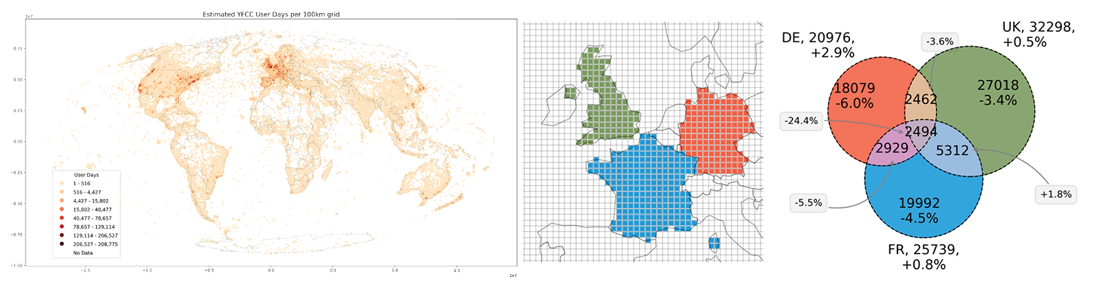
YFCC100M Example: Monitoring of Worldwide User Days
A User Day refers to a common metric used in visual analytics.
Each user is counted once per day.
This is commonly done by concatentation of a unique user identifier and the unique day of activity, e.g.:
userdays_set = set()
userday_sample = "96117893@N05" + "2012-04-14"
userdays_set.add(userday_sample)
print(len(userdays_set))
> 1
We have create an example processing pipeline for counting user days world wide, using the Flickr YFCC100M dataset, which contains about 50 Million georeferenced photos uploaded by Flickr users with a Creative Commons License.
The full processing pipeline can be viewed in a separate collection of notebooks.
In the following, we will use the HLL data to replicate these visuals.
We'll use python methods stored and loaded from modules.
Data collection granularity
There's a difference between collecting and visualizing data.
During data collection, information can be stored with a higher
information granularity, to allow some flexibility for
tuning visualizations.
In the YFCC100M Example, we "collect" data at a GeoHash granularity of 5
(about 3 km "snapping distance" for coordinates).
During data visualization, these coordinates and HLL sets are aggregated
further to a worldwide grid of 100x100 km bins.
Have a look at the data structure at data collection time.
from pathlib import Path

OUTPUT = Path.cwd() / "out"
OUTPUT.mkdir(exist_ok=True)
%load_ext autoreload
%autoreload 2
import sys

module_path = str(Path.cwd().parents[0] / "py")
if module_path not in sys.path:
    sys.path.append(module_path)
from modules import tools
Load the full benchmark dataset.
filename = "yfcc_latlng.csv"
yfcc_input_csv_path = OUTPUT / filename
if not yfcc_input_csv_path.exists():
    sample_url = tools.get_sample_url()
    yfcc_csv_url = f'{sample_url}/download?path=%2F&files={filename}'
    tools.get_stream_file(url=yfcc_csv_url, path=yfcc_input_csv_path)
Load csv data to pandas dataframe.
%%time
import pandas as pd
dtypes = {'latitude': float, 'longitude': float}
df = pd.read_csv(
    OUTPUT / "yfcc_latlng.csv", dtype=dtypes, encoding='utf-8')
print(len(df))
The dataset contains a total number of 451,949 distinct coordinates,
at a GeoHash precision of 5 (~2500 Meters snapping distance.)
df.head()
Calculate a single HLL cardinality (first row):
sample_hll_set = df.loc[0, "date_hll"]
from python_hll.util import NumberUtil
hex_string = sample_hll_set[2:]
print(sample_hll_set[2:])
hll = HLL.from_bytes(NumberUtil.from_hex(hex_string, 0, len(hex_string)))
hll.cardinality()
The two components of the structure are highlighted below.
tools.display_header_stats(
    df.head(),
    base_cols=["latitude", "longitude"],
    metric_cols=["date_hll"])
The color refers to the two components:
Compare RAW data
- Unlike RAW data, the user-id and the distinct dates are stored in the HLL sets above (date_hll)
- When using RAW data, storing the user-id and date, to count userdays, would also mean
that each user can be tracked across different locations and times - HLL allows to prevent such misuse of data.
Data visualization granularity
- there're many ways to visualize data
- typically, visualizations will present
information at a information granularity
that is suited for the specific application
context - To aggregate information from HLL data,
individual HLL sets need to be merged
(a union operation) - For the YFCC100M Example, the process
to union HLL sets is shown here - We're going to load and visualize this
aggregate data below
from modules import yfcc
filename = "yfcc_all_est_benchmark.csv"
yfcc_benchmark_csv_path = OUTPUT / filename
if not yfcc_benchmark_csv_path.exists():
    yfcc_csv_url = f'{sample_url}/download?path=%2F&files={filename}'
    tools.get_stream_file(
        url=yfcc_csv_url, path=yfcc_benchmark_csv_path)
grid = yfcc.grid_agg_fromcsv(
    OUTPUT / filename,
    columns=["xbin", "ybin", "userdays_hll"])
grid[grid["userdays_hll"].notna()].head()
tools.display_header_stats(
    grid[grid["userdays_hll"].notna()].head(),
    base_cols=["geometry"],
    metric_cols=["userdays_hll"])
Description of columns
- geometry: A WKT-Polygon for the area (100x100km bin)
- userdays_hll: The HLL set, containing all userdays measured for the respective area
- xbin/ybin: The DataFrame (multi-) index, each 100x100km bin has a unique x and y number.
Calculate the cardinality for all bins and store in extra column:
def hll_from_byte(hll_set: str):
    """Return HLL set from binary representation"""
    hex_string = hll_set[2:]
    return HLL.from_bytes(
        NumberUtil.from_hex(
            hex_string, 0, len(hex_string)))
def cardinality_from_hll(hll_set):
    """Turn binary hll into HLL set and return cardinality"""
    hll = hll_from_byte(hll_set)
    return hll.cardinality() - 1
Calculate cardinality for all bins.
This process will take some time (about 3 Minutes),
due to using slow python-hll implementation.
%%time
mask = grid["userdays_hll"].notna()
grid["userdays_est"] = 0
grid.loc[mask, 'userdays_est'] = grid[mask].apply(
        lambda x: cardinality_from_hll(
           x["userdays_hll"]),
        axis=1)
RuntimeWarning?
- python-hll library is in a very early stage of development
- it is not fully compatible with the citus hll implementation in postgres
- The shown RuntimeWarning (Overflow) is one of the issues that need to be resolved in the future
- If you run this notebook locally, it is recommended to use pg-hll-empty for any hll calculations, as is shown (e.g.) in the original YFCC100M notebooks.
grid[mask].apply()?
- This is another example of boolean masking with pandas
grid["userdays_hll"].notna()creates a list (apd.Series) of True/False valuesgrid.loc[mask, 'userdays_est']uses the index of the mask, to select indexes, and the column 'userdays_est', to assign values
From now on, disable warnings:
import warnings
warnings.filterwarnings('ignore')
Have a look at the cardinality below.
grid[grid["userdays_hll"].notna()].head()
Visualize the grid, using prepared methods
Activate the bokeh holoviews extension.
from modules import grid as yfcc_grid
import holoviews as hv
hv.notebook_extension('bokeh')


.. visualize the grid, as an interactive map, shown in the notebook:
gv_layers = yfcc_grid.plot_interactive(
    grid, title=f'YFCC User Days (estimated) per 100 km grid',
    metric="userdays_est")
gv_layers
.. or, store as an external HTML file, to be viewed separately:
yfcc_grid.plot_interactive(
    grid, title=f'YFCC User Days (estimated) per 100 km grid', metric="userdays_est",
    store_html="yfcc_userdays_est", output=OUTPUT)
Open HTML
- go to notebooks/out
- .. and open yfcc_userdays_est.html with
Right-Click > Open In New Browser-Tab
Working with HLL data: Intersection Example
HLL is not pure statistic data.
There is some flexibility to explore HLL sets further,
by using the union and intersection functionality.
We're going to explore this functionality below.
The task is to union all HLL sets for userdays for:
- Germany
- France
- UK
.. and finally visualizing total user counts for these countries
and the subset of users that have visited two or all of these
countries.
Python GIS Operations
- The code below is not any more complex than working with RAW data
- We'll learn how to use some common GIS operations in python below
Why user counts, and not user days?
- Userdays (eg. in the form of
user-id||date) are not suited to study visitation intersection between countries. - In other words, it is unlikely that one user has visited more than one country on a single day.
- No or little intersection would be found by using user days.
- Using hashed user ids (converted to HLL) instead allows to count the users having visited two or more countries
Load user hll sets:
grid = yfcc.grid_agg_fromcsv(
    OUTPUT / "yfcc_all_est_benchmark.csv",
    columns=["xbin", "ybin", "usercount_hll"])
Preview:
grid[grid["usercount_hll"].notna()].head()
Union hll sets for Countries UK, DE and FR
Selection of grid cells based on country geometry
Load country geometry:
import geopandas as gp
world = gp.read_file(
    gp.datasets.get_path('naturalearth_lowres'),
    crs=yfcc.CRS_WGS)
world = world.to_crs(
    yfcc.CRS_PROJ)
gp.datasets.get_path()?
- Some data is provided by Geopandas
- One of these datasets is the natural earth lowres countries shapefile
- .. but you can load any Shapefile or GIS data here.
Select geometry for DE, FR and UK
de = world[world['name'] == "Germany"]
uk = world[world['name'] == "United Kingdom"]
fr = world[world['name'] == "France"]
Select different countries
- Optionally: Modify the list of countries to adapt visualizations below.
Drop French territory of French Guiana:
fr = fr.explode().iloc[1:].dissolve(by='name')
fr.plot()

Preview selection.
Note that the territory of France includes Corsica,
which is acceptable for the example use case.
import matplotlib.pyplot as plt
fig, (ax1, ax2, ax3) = plt.subplots(1, 3)
fig.suptitle(
    'Areas to test for common visitors in the hll benchmark dataset')
for ax in (ax1, ax2, ax3):
    ax.set_axis_off()
ax1.title.set_text('DE')
ax2.title.set_text('UK')
ax3.title.set_text('FR')
de.plot(ax=ax1)
uk.plot(ax=ax2)
fr.plot(ax=ax3)

Intersection with grid
Since grid size is 100 km,
direct intersection will yield some error rate (in this case, called _MAUP_).
Use centroid of grid cells to select bins based on country geometry.
Get centroids as Geoseries and turn into GeoDataFrame:
centroid_grid = grid.centroid.reset_index()
centroid_grid.set_index(["xbin", "ybin"], inplace=True)
grid.centroid
Define function to intersection, using geopandas sjoin (spatial join)
from geopandas.tools import sjoin
def intersect_grid_centroids(
    grid: gp.GeoDataFrame,
    intersect_gdf: gp.GeoDataFrame):
    """Return grid centroids from grid that
    intersect with intersect_gdf
    """
    centroid_grid = gp.GeoDataFrame(
        grid.centroid)
    centroid_grid.rename(
        columns={0:'geometry'},
        inplace=True)
    centroid_grid.set_geometry(
        'geometry', crs=grid.crs,
        inplace=True)
    grid_intersect = sjoin(
        centroid_grid, intersect_gdf,
        how='right')
    grid_intersect.set_index(
        ["index_left0", "index_left1"],
        inplace=True)
    grid_intersect.index.names = ['xbin','ybin']
    return grid.loc[grid_intersect.index]
Run intersection for countries:
grid_de = intersect_grid_centroids(
    grid=grid, intersect_gdf=de)
grid_de.plot(edgecolor='white')

grid_fr = intersect_grid_centroids(
    grid=grid, intersect_gdf=fr)
grid_fr.plot(edgecolor='white')

grid_uk = intersect_grid_centroids(
    grid=grid, intersect_gdf=uk)
grid_uk.plot(edgecolor='white')

Plot preview of selected grid cells (bins)
Define colors:
color_de = "#fc4f30"
color_fr = "#008fd5"
color_uk = "#6d904f"
Define map boundary:
bbox_europe = (
    -9.580078, 41.571384,
    16.611328, 59.714117)
minx, miny = yfcc.PROJ_TRANSFORMER.transform(
    bbox_europe[0], bbox_europe[1])
maxx, maxy = yfcc.PROJ_TRANSFORMER.transform(
    bbox_europe[2], bbox_europe[3])
buf = 100000
from typing import List, Optional
def plot_map(
    grid: gp.GeoDataFrame, sel_grids: List[gp.GeoDataFrame],
    sel_colors: List[str],
    title: Optional[str] = None, save_fig: Optional[str] = None,
    ax = None, output: Optional[Path] = OUTPUT):
    """Plot GeoDataFrame with matplotlib backend, optionaly export as png"""
    if not ax:
        fig, ax = plt.subplots(1, 1, figsize=(5, 6))
    ax.set_xlim(minx-buf, maxx+buf)
    ax.set_ylim(miny-buf, maxy+buf)
    if title:
        ax.set_title(title, fontsize=12)
    for ix, sel_grid in enumerate(sel_grids):
        sel_grid.plot(
            ax=ax,
            color=sel_colors[ix],
            edgecolor='white',
            alpha=0.9)
    grid.boundary.plot(
        ax=ax,
        edgecolor='black',
        linewidth=0.1,
        alpha=0.9)
    # combine with world geometry
    world.plot(
        ax=ax, color='none', edgecolor='black', linewidth=0.3)
    # turn axis off
    ax.set_axis_off()
    if not save_fig:
        return
    fig.savefig(output / save_fig, dpi=300, format='PNG',
               bbox_inches='tight', pad_inches=1)
sel_grids=[grid_de, grid_uk, grid_fr]
sel_colors=[color_de, color_uk, color_fr]
plot_map(
    grid=grid, sel_grids=sel_grids,
    sel_colors=sel_colors,
    title='Grid selection for DE, FR and UK',
    save_fig='grid_selection_countries.png')

Union of hll sets
def union_hll(hll: HLL, hll2):
    """Union of two HLL sets. The first HLL set will be modified in-place."""
    hll.union(hll2)

def union_all_hll(
    hll_series: pd.Series, cardinality: bool = True) -> pd.Series:
    """HLL Union and (optional) cardinality estimation from series of hll sets

        Args:
        hll_series: Indexed series (bins) of hll sets.
        cardinality: If True, returns cardinality (counts). Otherwise,
            the unioned hll set will be returned.
    """

    hll_set = None
    for hll_set_str in hll_series.values.tolist():
        if hll_set is None:
            # set first hll set
            hll_set = hll_from_byte(hll_set_str)
            continue
        hll_set2 = hll_from_byte(hll_set_str)
        union_hll(hll_set, hll_set2)
    return hll_set.cardinality()
Calculate distinct users per country:
grid_sel = {
    "de": grid_de,
    "uk": grid_uk,
    "fr": grid_fr
}
distinct_users_total = {}
for country, grid_sel in grid_sel.items():
    # drop bins with no values
    cardinality_total = union_all_hll(
        grid_sel["usercount_hll"].dropna())
    distinct_users_total[country] = cardinality_total
    print(
        f"{distinct_users_total[country]} distinct users "
        f"who shared YFCC100M photos in {country.upper()}")
Calculate intersection (common visitors)
According to the Union-intersection-principle:
$|A \cup B| = |A| + |B| - |A \cap B|$
which can also be written as:
$|A \cap B| = |A| + |B| - |A \cup B|$
Therefore, unions can be used to calculate intersection. Calculate $|DE \cup FR|$, $|DE \cup UK|$ and $|UK \cup FR|$, i.e.:
IntersectionCount =
hll_cardinality(grid_de)::int +
hll_cardinality(grid_fr)::int -
hll_cardinality(hll_union(grid_de, grid_fr)
First, prepare combination for different sets.
union_de_fr = pd.concat([grid_de, grid_fr])
union_de_uk = pd.concat([grid_de, grid_uk])
union_uk_fr = pd.concat([grid_uk, grid_fr])
Calculate union
grid_sel = {
    "de-uk": union_de_uk,
    "de-fr": union_de_fr,
    "uk-fr": union_uk_fr
}
distinct_common = {}
for country_tuple, grid_sel in grid_sel.items():
    cardinality = union_all_hll(
        grid_sel["usercount_hll"].dropna())
    distinct_common[country_tuple] = cardinality
    print(
        f"{distinct_common[country_tuple]} distinct total users "
        f"who shared YFCC100M photos from either {country_tuple.split('-')[0]} "
        f"or {country_tuple.split('-')[1]} (union)")
Calculate intersection
distinct_intersection = {}
for a, b in [("de", "uk"), ("de", "fr"), ("uk", "fr")]:
    a_total = distinct_users_total[a]
    b_total = distinct_users_total[b]
    common_ref = f'{a}-{b}'
    intersection_count = a_total + b_total - distinct_common[common_ref]
    distinct_intersection[common_ref] = intersection_count
    print(
        f"{distinct_intersection[common_ref]} distinct users "
        f"who shared YFCC100M photos from {a} and {b} (intersection)")
Finally, lets get the number of users who have shared pictures from all three countries, based on the formula for three sets:
$|A \cup B \cup C| = |A| + |B| + |C| - |A \cap B| - |A \cap C| - |B \cap C| + |A \cap B \cap C|$
which can also be written as:
$|A \cap B \cap C| = |A \cup B \cup C| - |A| - |B| - |C| + |A \cap B| + |A \cap C| + |B \cap C|$
Calculate distinct users of all three countries:
union_de_fr_uk = pd.concat(
    [grid_de, grid_fr, grid_uk])
cardinality = union_all_hll(
    union_de_fr_uk["usercount_hll"].dropna())
union_count_all = cardinality
union_count_all
country_a = "de"
country_b = "uk"
country_c = "fr"
Calculate intersection
intersection_count_all = union_count_all - \
    distinct_users_total[country_a] - \
    distinct_users_total[country_b] - \
    distinct_users_total[country_c] + \
    distinct_intersection[f'{country_a}-{country_b}'] + \
    distinct_intersection[f'{country_a}-{country_c}'] + \
    distinct_intersection[f'{country_b}-{country_c}']

print(intersection_count_all)
Visualize intersection using Venn diagram
Since we're going to visualize this with matplotlib-venn, we need the following variables:
from matplotlib_venn import venn3, venn3_circles
v = venn3(
    subsets=(
        500,
        500,
        100,
        500,
        100,
        100,
        10),
    set_labels = ('A', 'B', 'C'))
v.get_label_by_id('100').set_text('Abc')
v.get_label_by_id('010').set_text('aBc')
v.get_label_by_id('001').set_text('abC')
v.get_label_by_id('110').set_text('ABc')
v.get_label_by_id('101').set_text('AbC')
v.get_label_by_id('011').set_text('aBC')
v.get_label_by_id('111').set_text('ABC')
plt.show()

We already have ABC, the other values can be calulated:
ABC = intersection_count_all
ABc = distinct_intersection[f'{country_a}-{country_b}'] - ABC
aBC = distinct_intersection[f'{country_b}-{country_c}'] - ABC
AbC = distinct_intersection[f'{country_a}-{country_c}'] - ABC
Abc = distinct_users_total[country_a] - ABc - AbC + ABC
aBc = distinct_users_total[country_b] - ABc - aBC + ABC
abC = distinct_users_total[country_c] - aBC - AbC + ABC
Illustrate intersection (Venn diagram)
Order of values handed over: Abc, aBc, ABc, abC, AbC, aBC, ABC
Define Function to plot Venn Diagram.
from typing import Tuple

def plot_venn(
    subset_sizes: List[int],
    colors: List[str],
    names: List[str],
    subset_sizes_raw: List[int] = None,
    total_sizes: List[Tuple[int, int]] = None,
    ax = None,
    title: str = None):
    """Plot Venn Diagram"""
    if not ax:
        fig, ax = plt.subplots(1, 1, figsize=(5,5))
    set_labels = (
        'A', 'B', 'C')
    v = venn3(
        subsets=(
            [subset_size for subset_size in subset_sizes]),
        set_labels = set_labels,
        ax=ax)
    for ix, idx in enumerate(
        ['100', '010', '001']):
        v.get_patch_by_id(
            idx).set_color(colors[ix])
        v.get_patch_by_id(
            idx).set_alpha(0.8)
        v.get_label_by_id(
            set_labels[ix]).set_text(
            names[ix])
        if not total_sizes:
            continue
        raw_count = total_sizes[ix][0]
        hll_count = total_sizes[ix][1]
        difference = abs(raw_count-hll_count)
        v.get_label_by_id(set_labels[ix]).set_text(
            f'{names[ix]}, {hll_count},\n'
            f'{difference/(raw_count/100):+.1f}%')
    if subset_sizes_raw:
        for ix, idx in enumerate(
            ['100', '010', None, '001']):
            if not idx:
                continue
            dif_abs = subset_sizes[ix] - subset_sizes_raw[ix]
            dif_perc = dif_abs / (subset_sizes_raw[ix] / 100)
            v.get_label_by_id(idx).set_text(
                f'{subset_sizes[ix]}\n{dif_perc:+.1f}%')
    label_ids = [
        '100', '010', '001',
        '110', '101', '011',
        '111', 'A', 'B', 'C']
    for label_id in label_ids:
        v.get_label_by_id(
            label_id).set_fontsize(14)
    # draw borders
    c = venn3_circles(
        subsets=(
            [subset_size for subset_size in subset_sizes]),
        linestyle='dashed',
        lw=1,
        ax=ax)
    if title:
        ax.title.set_text(title)
Plot Venn Diagram:
subset_sizes = [
    Abc, aBc, ABc, abC, AbC, aBC, ABC]
colors = [
    color_de, color_uk, color_fr]
names = [
    'Germany', 'United Kingdom','France']
plot_venn(
    subset_sizes=subset_sizes,
    colors=colors,
    names=names,
    title="Common User Count")

Combine Map & Venn Diagram
# figure with subplot (1 row, 2 columns)
fig, ax = plt.subplots(1, 2, figsize=(10, 24))
plot_map(
    grid=grid, sel_grids=sel_grids,
    sel_colors=sel_colors, ax=ax[0])
plot_venn(
    subset_sizes=subset_sizes,
    colors=colors,
    names=names,
    ax=ax[1])
# store as png
fig.savefig(
    OUTPUT / "hll_intersection_ukdefr.png", dpi=300, format='PNG',
    bbox_inches='tight', pad_inches=1)

Error rates
- Guaranteed error rates (2-3%) apply to HLL any union operation
- When intersecting HLL sets, error rates may increase, depending on the size of sets
- This is a limitation, but also provides a protection that prevents identifying individual users through intersection
- Have a look at the YFCC100M paper notebook, where we have created the Venn diagram with raw and hll data, illustrating error rates
Create Notebook HTML
Save the Notebook, then execute the following cell to convert to HTML (archive format).
!jupyter nbconvert --to html \
    --output-dir=./out/ ./02_hll_intro.ipynb \
    --template=../nbconvert.tpl \
    --ExtractOutputPreprocessor.enabled=False >&- 2>&-
Summary
Notes
- Python-hll, the lbsn structure and other tools shown in this work are in an early stage of development
- Adaption of workflows to the privacy-aware data structure requires effort
- Many, but not all visualizations are suited to be used with HLL data
- The lbsn structure is a convention, there're many different ways to use and apply HLL in visual analytics. With the structure, we have specifically looked at the utility of HLL to privacy.
Further work
- Have a look at the tutorial section
- Try to replicate the Minimal example, which explains how to start
rawdbandhlldblocally using Docker - Clone and run YFCC100M grid aggregation notebooks, which demonstrate the full pipeline of importing, processing and visualizing data