Part 3: Tag Maps Clustering and Topic Heat Maps

Workshop: Social Media, Data Science, & Cartograpy
Alexander Dunkel, Madalina Gugulica

This is the third notebook in a series of four notebooks:

1. Introduction to Social Media data, jupyter and python spatial visualizations
2. Introduction to privacy issues with Social Media data and possible solutions for cartographers
3. Specific visualization techniques example: TagMaps clustering
4. Specific data analysis: Topic Classification

Open these notebooks through the file explorer on the left side.

Introduction: Privacy & Social Media

The task in this notebook is to extract and visualize common areas or regions of interest for a given topic from Location Based Social Media data (LBSM).

On Social Media, people react to many things, and a significant share of these reactions can be seen as forms of valuation or attribution of meaning to to the physical environment.

Challenges

However, for visualizing such values for whole cities, there are several challenges involved:

• Identify reactions that are related to a given topic:
• Topics can be considered at different levels of granularity
• and equal terms may convey different meanings in different contexts.
• Social Media data is distributed very irregularly.
• Data peaks in urban areas and highly frequented tourist hotspots,
• while some less frequented areas do not feature any data at all.
• When visualizing spatial reactions to topics, this unequal distribution must be taking into account, otherwise maps would always be biased towards areas with higher density of information.
• For this reason, normalizing results is crucial.
• The usual approach for normalization in such cases is that local distribution is evaluated against the global (e.g. spatial) distribution data.

Tag Maps Package

• The Tag Maps package was developed to cluster tags according to their spatial area of use
• Currently, the final visualization step of Tag Maps clustering (placing labels etc.) is only implemented in ArcMap
• Herein, we instead explore cluster results using Heat Maps and other graphics in python
• In the second part of the workshop, it will be shown how to visualize the actual Tag Maps

Where is my custom area/tag map?

• Below, you can chose between different regions/areas to explore in this notebook, provided based on student input
• The final Tag Map visualization step is currently not possible in Jupyter/Python
• We will meet at the end of January in the GeoPool, to visualize custom areas using ArcMap

Important:

• The privacy-aware data structure shown in the second Notbook has not been implemented yet in tag maps
• We will be working with RAW data instead
• Please:
• Do not share the original data
• Remove original data after the workshop

Preparations

Define output directory

from pathlib import Path
OUTPUT = Path.cwd() / "out"

Load the TagMaps package, which will serve as a base for filtering, cleaning and processing noisy social media data

from tagmaps import TagMaps
from tagmaps import EMOJI, TAGS, TOPICS
from tagmaps import LoadData
from tagmaps import BaseConfig

Load Data & Plot Overview

Create 01_Input folder, which will be used for loading data.

INPUT = Path.cwd() / "01_Input"

Retrieve sample LBSN CSV data:

%load_ext autoreload
%autoreload 2

The autoreload extension is already loaded. To reload it, use:
  %reload_ext autoreload

import sys

module_path = str(Path.cwd().parents[0] / "py")
if module_path not in sys.path:
    sys.path.append(module_path)
from modules import tools

source = "GrosserGarten.zip"
# source = "Jadavpur.zip"
# source = "Istanbul.zip"
# source = "Tokio.zip"
# source = "Kazan.zip"
# source = "Lindau.zip"
# source = "Hasenheide.zip"
# source = "tumunich.zip"

Select Input

• Based on requests, we have provided several sources of data
• Choose one of the input source above
• The default input data is for the Großer Garten in Dresden

%%time
# clean any data first
tools.clean_folders([INPUT])
sample_url = tools.get_sample_url()
lbsn_dd_csv_uri = f'{sample_url}/download?path=%2F&files='
tools.get_zip_extract(
    uri=lbsn_dd_csv_uri,
    filename=source,
    output_path=INPUT,
    write_intermediate=True)

Cancel.
Done. Thank you. Do not forget to shut down your notebook server (File > Shut Down), once you are finished with the last notebook.
File already exists.. skipping download..
CPU times: user 48 ms, sys: 9.55 ms, total: 57.6 ms
Wall time: 7.25 s

Initialize tag maps from BaseConfig

tm_cfg = BaseConfig()

Loaded 337 stoplist items.
Loaded 214 inStr stoplist items.
Loaded 4 stoplist places.
Loaded 3 place lat/lng corrections.

Optionally, filter data per origin or adjust the number of top terms to extract:

tm_cfg.filter_origin = None
tm_cfg.max_items = 3000

tm_opts = {
    'tag_cluster':tm_cfg.cluster_tags,
    'emoji_cluster':tm_cfg.cluster_emoji,
    'location_cluster':tm_cfg.cluster_locations,
    'output_folder':tm_cfg.output_folder,
    'remove_long_tail':tm_cfg.remove_long_tail,
    'limit_bottom_user_count':tm_cfg.limit_bottom_user_count,
    'max_items':tm_cfg.max_items,
    'topic_cluster':True}
tm = TagMaps(**tm_opts)

**kwargs syntax?

• Some functions take a long list of (keyword) arguments
• These keyword arguments can be passed to the function using a dictionary
• The ** syntax tells python to unpack keyword arguments from a dictionary

a) Read from original data

Read input records from csv

from IPython.display import clear_output

%%time
input_data = LoadData(tm_cfg)
with input_data as records:
    for ix, record in enumerate(records):
        tm.add_record(record)
        if (ix % 1000) != 0:
            continue
        # report every 1000 records
        clear_output(wait=True)
        print(f'Loaded {ix} records')
input_data.input_stats_report()
tm.prepare_data()

Loaded 244000 records
Cleaned input to 18229 distinct locations from 244942 posts (File 2 of 2) - Skipped posts: 0 - skipped tags: 146435 of 1596294

Total post count (PC): 244942
Total tag count (PTC): 1596294
Total emoji count (PEC): 167916
Long tail removal: Filtered 385 Emoji that were used by less than 2 users.
Long tail removal: Filtered 157643 Topics that were used by less than 5 users.
CPU times: user 1min 18s, sys: 1.4 s, total: 1min 19s
Wall time: 1min 18s

b) Optional: Write (& Read) cleaned output to file

Output cleaned data to Output/Output_cleaned.csv,
clean terms (post_body and tags) based on the top (e.g.) 1000 hashtags found in dataset.

tm.lbsn_data.write_cleaned_data(panon=True)

Writing cleaned intermediate data to file (Output_cleaned.csv)..
 done.

Have a look at the output file.

import pandas as pd

file_path = Path.cwd() / "02_Output" / "Output_cleaned.csv"
display(pd.read_csv(file_path, nrows=5).head())
print(f'{file_path.stat().st_size / (1024*1024):.02f} MB')

	origin_id	lat	lng	guid	user_guid	loc_id	post_create_date	post_publish_date	post_body	hashtags	emoji	post_views_count	post_like_count	loc_name
0	1	51.033300	13.733300	3722a733575bfbd6c173dc2deadb795b	3722a733575bfbd6c173dc2deadb795b	51.0333:13.7333	NaN	NaN	fürstenzug	NaN	NaN	704	0	Fürstenzug
1	1	51.033300	13.733300	ac28e6f721e25624d76a9eb3afc61b4f	ac28e6f721e25624d76a9eb3afc61b4f	51.0333:13.7333	NaN	NaN	NaN	NaN	NaN	194	0	Hochschulstraße
2	1	51.033300	13.733300	d71246d019402566900f0d59d0c9fbef	d71246d019402566900f0d59d0c9fbef	51.0333:13.7333	NaN	NaN	stadtfest;dresdner	NaN	NaN	181	0	Dresdner Stadtfest
3	1	51.031945	13.730668	0ff8be1630ab8decae97efecfda9f5f3	0ff8be1630ab8decae97efecfda9f5f3	51.031945353:13.7306680064	NaN	NaN	club	NaN	NaN	228	0	Club 11
4	1	51.031224	13.730091	aab11415bd4546adef5f513ac00edc90	aab11415bd4546adef5f513ac00edc90	51.0312241:13.7300907	NaN	NaN	house;international	NaN	NaN	66	0	International Guest House

46.03 MB

Data Minimization

• The cleaned output file is significantly smaller than original data
• It includes only a small subset of original terms, based on filtering of frequently used terms
• As a minor precaution, IDs, such as guid or user_guid, have been pseudonymized.
• In reality, such pseudonymization will be easy to reverse, and thus only provides a minor protection to misuse of data

Read from pre-filtered data

Read data form (already prepared and filtered) cleaned output

%%time
tm.prepare_data(
    input_path=file_path)

CPU times: user 2.5 ms, sys: 16 µs, total: 2.51 ms
Wall time: 2.52 ms

tm.global_stats_report()
tm.item_stats_report()

Total user count (UC): 103684
Total user post locations (UPL): 168815
Number of locations with names: 2294
Total distinct tags (DTC): 174260
Total distinct emoji (DEC): 2078
Total distinct locations (DLC): 18229
Total tag count for the 3000 most used tags in selected area: 1778500.
Total emoji count for the 1693 most used emoji in selected area: 167487.
Bounds are: Min 13.727952 51.0257536334 Max 13.78818 51.051867

Topic selection & Tag Clustering

The next goal is to select reactions to given topics. TagMaps allows selecting posts for 4 different types:

• TAGS (i.e. single terms)
• EMOJI (i.e. single emoji)
• LOCATIONS (i.e. named POIs or coordinate pairs)
• TOPICS (i.e. list of terms)

Set basic plot to notebook mode and disable interactive plots for now

import matplotlib.pyplot as plt
import matplotlib as mpl
%matplotlib inline
mpl.rcParams['savefig.dpi'] = 120
mpl.rcParams['figure.dpi'] = 120

We can retrieve preview maps for the TOPIC dimension
by supplying a list of terms.

For example "park", "green" and "grass" should
give us an overview where such terms are used
in our sample area.

Custom topic

• Try to process first with the supplied set of terms
• Afterwards, choose your own set of terms to affect visualizations below
• You can repeat the process for different topics by starting in this cell again

nature_terms = ["park", "grass", "nature"]
fig = tm.get_selection_map(
    TOPICS, nature_terms)

urban_terms = ["strasse", "city", "shopping"]
fig = tm.get_selection_map(
    TOPICS, urban_terms)

HDBSCAN Cluster

We can visualize clusters for the selected topic using HDBSCAN.

The important parameter for HDBSCAN is the cluster distance,
which is chosen automatically by Tag Maps given the current scale/extent of analysis.

# tm.clusterer[TOPICS].cluster_distance = 150
fig = tm.get_cluster_map(
    TOPICS, nature_terms)

Manually select cluster distance

• TagMaps automatically selects a suitable cluster distance
• For the Großer Garten dataset, this distance is 203 meters
• We can select a smaller cluster distance, to get finer grained picture of topic clusters.
• In the cell above, uncomment the first line and re-run the cell
• Try other cluster distances to see how the output changes.

We can get a map of clusters and cluster shapes (convex and concave hulls).

fig = tm.get_cluster_shapes_map(
    TOPICS, nature_terms)

--> 31 cluster.

Behind the scenes, Tag Maps utilizes the Single Linkage Tree from HDBSCAN to cut clusters at a specified distance. This tree shows the hierarchical structure for our topic and its spatial properties in the given area.

fig = tm.get_singlelinkagetree_preview(
    TOPICS, nature_terms)

Cluster centroids

Similarly, we can retrieve centroids of clusters. This shows again the unequal distribution of data:

fig = tm.clusterer[TOPICS].get_cluster_centroid_preview(
    nature_terms, single_clusters=True)

(1 of 16617) Found 2928 posts (UPL) for Topic 'park-grass-nature' (found in 6% of DLC in area) --> 31 cluster.

Heat Maps

• Visualization of clustered tagmaps data is possible in several ways.
• In the second workshop (end of January), we are using ArcMap, to create labeled maps from clustered data
• The last part in this notebook will be to use Kernel Densitry Estimation (KDE) to create a Heat Map for selected topics.

Further information: KDE

• Some of the code below was adapted from plot species example
• A more thorough tutorial is provided here
• The Python Data Science Handbook also contains a section on KDE

Import dependencies

import numpy as np
from sklearn.neighbors import KernelDensity

Load Flickr data only

Instagram, Facebook and Twitter are based on place-accuracy, which is unsuitable for the Heat Map graphic.

We'll work with Flickr data only for the Heat Map.

• 1 = Instagram
• 2 = Flickr
• 3 = Twitter

Reload data, filtering only Flickr

tm_cfg.filter_origin = "2"
tm = TagMaps(**tm_opts)

%%time
input_data = LoadData(tm_cfg)
with input_data as records:
    for ix, record in enumerate(records):
        tm.add_record(record)
        if (ix % 1000) != 0:
            continue
        # report every 1000 records
        clear_output(wait=True)
        print(f'Loaded {ix} records')
input_data.input_stats_report()

Loaded 31000 records
Cleaned input to 15951 distinct locations from 31309 posts (File 2 of 2) - Skipped posts: 213572 - skipped tags: 36969 of 232936

Total post count (PC): 31309
Total tag count (PTC): 232936
Total emoji count (PEC): 0
CPU times: user 7.83 s, sys: 246 ms, total: 8.08 s
Wall time: 7.95 s

Get Topic Coordinates

The distribution of these coordinates is what we want to visualize.

tm.prepare_data()
tm.init_cluster()

Long tail removal: Filtered 1959 Tags that were used by less than 5 users.
Long tail removal: Filtered 13164 Topics that were used by less than 5 users.

Topic selection

topic = "grass-nature-park"
points = tm.clusterer[TOPICS].get_np_points(
    item=topic,
    silent=True)

Why a different syntax? (term-term-term)

• The API of tagmaps package is still in an early stage
• The above function uses the internal representation of topics

Get All Points

all_points = tm.clusterer[TOPICS].get_np_points()

For normalizing our final KDE raster, we'll process both, topic selection points and global data distribution (e.g. all points in the dataset).

points_list = [points, all_points]

• The input data is a simply list (as a numpy.ndarray) of decimal degree coordinates
• each entry represents a single user that published one or more posts at a specific coordinate

print(points[:5])
print(f'Total coordinates: {len(points)}')

[[13.766544 51.036369]
 [13.755054 51.039289]
 [13.753187 51.043785]
 [13.762543 51.037939]
 [13.753069 51.038263]]
Total coordinates: 788

Data projection

• For faster KDE, we project data from WGS1984 (epsg:4326) to UTM
• this allows us to directly calculate in euclidian space.
• The TagMaps package automatically detected the most suitable UTM coordinate system,
• for the Großer Garten sample data, this is Zone 33N (epsg:32633)

Project lat/lng to UTM 33N (Dresden) using Transformer:

%%time
for idx, points in enumerate(points_list):
    points_list[idx] = np.array(
        [tm.clusterer[TOPICS].proj_transformer.transform(
                point[0], point[1]
        ) for point in points])
    
crs_wgs = tm.clusterer[TOPICS].crs_wgs
crs_proj = tm.clusterer[TOPICS].crs_proj
print(f'From {crs_wgs} \nto {crs_proj}')
print(points_list[0][:5])

From epsg:4326 
to epsg:32633
[[ 413517.95931985 5654593.12815275]
 [ 412717.86708307 5654931.37875778]
 [ 412595.43876854 5655433.54329967]
 [ 413240.37616266 5654772.41458472]
 [ 412576.773973   5654819.64201159]]
CPU times: user 101 ms, sys: 2.03 ms, total: 103 ms
Wall time: 99.9 ms

Calculating the Kernel Density

To summarize sklearn, a KDE is executed in two steps, training and testing:

Machine learning is about learning some properties of a data set and then testing those properties against another data set. A common practice in machine learning is to evaluate an algorithm by splitting a data set into two. We call one of those sets the training set, on which we learn some properties; we call the other set the testing set, on which we test the learned properties.

The only attributes we care about in training are lat and long.

• Stack locations using np.vstack, extract specific columns with [:,column_id]
• reverse order: lat, lng
• Transpose to Rows (.T), easier in python ref

xy_list = list()
for points in points_list:
    y = points[:, 1]
    x = points[:, 0]
    xy_list.append([x, y])

xy_train_list = list()
for x, y in xy_list:
    xy_train = np.vstack([y, x]).T
    xy_train_list.append(xy_train)

print(xy_train)

[[5655179.58377207  410936.28180054]
 [5655165.53133718  411138.62987412]
 [5655075.84309172  411088.98040009]
 ...
 [5655302.64257714  411360.89388318]
 [5654864.8466037   411463.97303812]
 [5655317.87392501  411322.44768116]]

Get bounds from total data

Access min/max decimal degree bounds object of clusterer and project to UTM33N

lim_lng_max = tm.clusterer[TAGS].bounds.lim_lng_max
lim_lng_min = tm.clusterer[TAGS].bounds.lim_lng_min
lim_lat_max = tm.clusterer[TAGS].bounds.lim_lat_max
lim_lat_min = tm.clusterer[TAGS].bounds.lim_lat_min

# project WDS1984 to UTM
topright = tm.clusterer[TOPICS].proj_transformer.transform(
    lim_lng_max, lim_lat_max)
bottomleft = tm.clusterer[TOPICS].proj_transformer.transform(
    lim_lng_min, lim_lat_min)

# get separate min/max for x/y
right_bound = topright[0]
left_bound = bottomleft[0]
top_bound = topright[1]
bottom_bound = bottomleft[1]

Create Sample Mesh

Create a grid of points at which to predict.

xbins=100j
ybins=100j
xx, yy = np.mgrid[
    left_bound:right_bound:xbins, 
    bottom_bound:top_bound:ybins]

xy_sample = np.vstack([yy.ravel(), xx.ravel()]).T

Generate Training data for Kernel Density.

• The largest effect on the final result comes from the chosen bandwidth for KDE - smaller bandwidth mean higher resultion,
• but may not be suitable for the given density of data (e.g. results with low validity).
• Higher bandwidth will produce a smoother raster result, which may be too inaccurate for interpretation.

Modify bandwidth parameter

• The bandwidth affects the distance at which points are considered during KDE
• Test all cells below first with the given bandwidth (200 meters)
• Afterwards, come back to this cell and adjust backwidth
• Compare the effect on visualization

kde_list = list()
for xy_train in xy_train_list:
    kde = KernelDensity(
        kernel='gaussian', bandwidth=200, algorithm='ball_tree')
    kde.fit(xy_train)
    kde_list.append(kde)

score_samples() returns the log-likelihood of the samples

%%time
z_list = list()
for kde in kde_list:
    z_scores = kde.score_samples(xy_sample)
    z = np.exp(z_scores)
    z_list.append(z)

CPU times: user 7.34 s, sys: 9.42 ms, total: 7.35 s
Wall time: 7.33 s

Remove values below zero,
these are locations where selected topic is underrepresented, given the global KDE mean

for ix in range(0, 2):
    z_list[ix] = z_list[ix].clip(min=0)

Normalize z-scores to 1 to 1000 range for comparison

for idx, z in enumerate(z_list):
    z_list[idx] = np.interp(
        z, (z.min(), z.max()), (1, 1000))

Subtact global zscores from local z-scores (our topic selection)

norm_val:

• weight of global z-score
• lower means less normalization effect, higher means stronger normalization effect
• range: 0 to 1

norm_val = 0.5
z_orig = z_list[0]
z_is = z_list[0] - (z_list[1]*norm_val)
z_results = [z_orig, z_is]

Modify norm_val parameter

• The normalization affects the the strength at which global values will have an effect on local values (the topic)
• Test all cells below first with the given normalization (0.5)
• Afterwards, come back to this cell and adjust normalization
• Compare the effect on visualization

Reshape results to fit grid mesh extent

for idx, z_result in enumerate(z_results):
    z_results[idx] = z_results[idx].reshape(xx.shape)

Plot original and normalized meshes

from matplotlib.ticker import FuncFormatter
def y_formatter(y_value, __):
    """Format UTM to decimal degrees y-labels for improved legibility"""
    xy_value = tm.clusterer[
        TOPICS].proj_transformer_back.transform(
            left_bound, y_value)
    return f'{xy_value[1]:3.2f}'

def x_formatter(x_value, __):
    """Format UTM to decimal degrees x-labels for improved legibility"""
    xy_value = tm.clusterer[
        TOPICS].proj_transformer_back.transform(
            x_value, bottom_bound)
    return f'{xy_value[0]:3.1f}'

# a figure with a 1x2 grid of Axes
fig, ax_lst = plt.subplots(1, 2, figsize=(10, 3))

for idx, zz in enumerate(z_results):
    axis = ax_lst[idx]
    # Change the fontsize of minor ticks label 
    axis.tick_params(axis='both', which='major', labelsize=7)
    axis.tick_params(axis='both', which='minor', labelsize=7)
    # set plotting bounds
    axis.set_xlim(
                [left_bound, right_bound])
    axis.set_ylim(
                [bottom_bound, top_bound])
    
    # plot contours of the density
    levels = np.linspace(zz.min(), zz.max(), 15)
    # Create Contours,
    # save to CF-variable so we can later reference
    # it in colorbar hook
    CF = axis.contourf(
        xx, yy, zz, levels=levels, cmap='viridis')
    # titles for plots
    if idx == 0:
        title = f'Original KDE for topic {topic}\n(Flickr Only)'
    else:
        title = f'Normalized KDE for topic {topic}\n(Flickr Only)'
    axis.set_title(title, fontsize=11)
    axis.set_xlabel('lng', fontsize=10)
    axis.set_ylabel('lat', fontsize=10)
    # plot points on top
    axis.scatter(
        xy_list[1][0], xy_list[1][1], s=1, facecolor='white', alpha=0.05)
    axis.scatter(
        xy_list[0][0], xy_list[0][1], s=1, facecolor='white', alpha=0.1)
    # replace x, y coords with decimal degrees text (instead of UTM dist)
    axis.yaxis.set_major_formatter(
        FuncFormatter(y_formatter))
    axis.xaxis.set_major_formatter(
        FuncFormatter(x_formatter))
    if idx > 0:
        break
    # Make a colorbar for the ContourSet returned by the contourf call.
    cbar = fig.colorbar(CF,fraction=0.046, pad=0.04)
    cbar.set_title = ""
    cbar.sup_title = ""
    cbar.ax.set_ylabel(
        "Number of \n User Post Locations (UPL)", fontsize=11)
    cbar.ax.set_title('')
    cbar.ax.tick_params(axis='both', labelsize=7)
    cbar.ax.yaxis.set_tick_params(width=0.5, length=4)

Depending on the data source and chosen topic, the two maps above will differ more or less.

For the Großer Garten Example and and nature topic,
the normalized map features little difference to the original KDE,
likely because there are little false positives in the surrounding area for nature reactions.

Combine HDBSCAN and KDE

For the final map, we want to combine the different data we collected.

This means adding cluster shapes from HDBSCAN and generating
a standalone interactive and external html for sharing.

from descartes import PolygonPatch
from tagmaps.classes.shared_structure import ItemCounter

def get_poly_patch(polygon):
    """Returns a matplotlib polygon-patch from shapely polygon"""
    patch = PolygonPatch(
        polygon, fc='#000000',
        ec='#999999', fill=False,
        zorder=1, alpha=0.7)
    return patch

Experimental code below

• Frequently, you will mix more production-ready code with experimental code cells in jupyter
• The code cell below is an example of experimental code:
• Things may change often here
• Only few code comments are provided
• A good recommendation is to put more effort into code that you will frequently re-use
• Once methods reach a certain maturity, store those in separate modules (e.g. the tools.py used herein)
• This allows you to re-use methods in other notebooks as well.

Modify cluster_distance parameter

• If you're working with other area datasets, adjust cluster_distance below to a suitable distance (meters)

fig, axis = plt.subplots(1)

# Change the fontsize of minor ticks label 
axis.tick_params(
    axis='both', which='major', labelsize=7)
axis.tick_params(
    axis='both', which='minor', labelsize=7)
# set plotting bounds
axis.set_xlim(
            [left_bound, right_bound])
axis.set_ylim(
            [bottom_bound, top_bound])

# plot contours of the density
levels = np.linspace(zz.min(), zz.max(), 25)
CF = axis.contourf(
    xx, yy, zz, levels=levels, cmap='viridis')

title = (f'Normalized KDE for topic {topic} '
         f'\n with HDBSCAN Cluster Shapes added '
         f'\n(Flickr Only)')
axis.set_title(title)
axis.set_xlabel('lng', fontsize=10)
axis.set_ylabel('lat', fontsize=10)
# plot points on top
axis.scatter(
    xy_list[0][0], xy_list[0][1],
    s=1, facecolor='white', alpha=0.1)
axis.yaxis.set_major_formatter(
    FuncFormatter(y_formatter))
axis.xaxis.set_major_formatter(
    FuncFormatter(x_formatter))

# Make a colorbar for the ContourSet 
# returned by the contourf call.
cbar = fig.colorbar(
    CF,
    label='Number of \n User Post Locations (UPL)',
    fraction=0.046, pad=0.04)
cbar.set_title = ""
cbar.sup_title = ""
cbar.ax.set_title('')
cbar.ax.tick_params(axis='both', labelsize=7)
cbar.ax.yaxis.set_tick_params(width=0.5, length=4)

# Get Cluster Shapes from TagMaps
tm.clusterer[TOPICS].cluster_distance = 200
result = tm.clusterer[TOPICS].cluster_item(
    item=topic,
    preview_mode=True)
clusters = result.clusters
selected_post_guids = result.guids

cluster_guids = tm.clusterer[TOPICS]._get_cluster_guids(
    clusters, selected_post_guids)
shapes = tm.clusterer[TOPICS]._get_item_clustershapes(
    ItemCounter(topic, 0), cluster_guids.clustered)
# create main cluster points map
for alpha_shape in shapes.alphashape:
    patch = get_poly_patch(alpha_shape.shape)
    axis.add_patch(patch)

--> 12 cluster.

Overlay Raster in Geoviews for interactive display

import holoviews as hv
import geoviews as gv
import geoviews.feature as gf
from cartopy.crs import epsg
import geoviews.tile_sources as gts
hv.notebook_extension('bokeh')

Get cartopy projection from epsg string.

cc_proj = epsg(
    crs_proj.split(":")[1])

Create contours from kde data

contours = gv.FilledContours(
    (xx.T, yy.T, zz.T),
    vdims='Number of \n User Post Locations (UPL)',
    crs=cc_proj)

Create additional layer for HDBSCAN cluster shapes

shape_list = [shape.shape for shape in shapes.alphashape]
gv_shapes = gv.Polygons(
    shape_list,
    label=f'HDBSCAN city-wide Cluster Shapes for topic',
    crs=cc_proj)

Prepare plotting

def set_active_tool(plot, element):
    """Enable wheel_zoom by default"""
    plot.state.toolbar.active_scroll = plot.state.tools[0]

Modify initial zoom extent

• The Overlay will automatically extent to data dimensions, the polygons of HDBSCAN cover the city area
• Since we want the initial zoom to be zoomed in to the Großer Garten we need to supply xlim and ylim.
• The Bokeh renderer only support Web Mercator Projection
• we therefore need to project Großer Garten Bounds first from WGS1984 to Web Mercator.
• We'll also zoom in from original max extents by about 50%

Prepare projection from WGS1984 to Web Mercator

from pyproj import Transformer

crs_proj = f"epsg:4326"
crs_wgs = "epsg:3857"

# define Transformer ahead of time
# with xy-order of coordinates
proj_transformer = Transformer.from_crs(
    crs_wgs, crs_proj, always_xy=True)

# also define reverse projection
proj_transformer_back = Transformer.from_crs(
    crs_proj, crs_wgs, always_xy=True)

Zoom in to 50% of original data extent

xcrop = (lim_lng_max - lim_lng_min) / 4
ycrop = (lim_lat_max - lim_lat_min) / 4
lim_lng_min_crop = lim_lng_min + xcrop
lim_lng_max_crop = lim_lng_max - xcrop
lim_lat_min_crop = lim_lat_min + ycrop
lim_lat_max_crop = lim_lat_max - ycrop

Apply transformation

gg_bottomleft = proj_transformer_back.transform(
    lim_lng_min_crop, lim_lat_min_crop)
gg_topright = proj_transformer_back.transform(
    lim_lng_max_crop, lim_lat_max_crop)

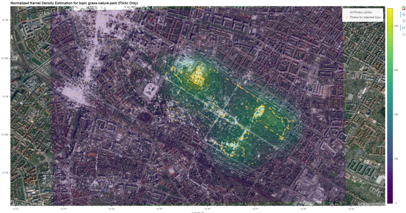
Construct final overlay from individual layers

1. Backgorund Tiles (sattelite)
2. All Points (Photos)
3. KDE Contours
4. Selected topic points ('green' photos)
5. HDBSCAN Cluster Shapes

bg_layer = gv.tile_sources.EsriImagery.opts(alpha=1.0)
all_photos_layer = gv.Points(
    (xy_list[1][0], xy_list[1][1]),
    label='All Photos (white)',
    crs=cc_proj).opts(size=5, color='white', alpha=0.3)
contours_layer = contours.opts(
    colorbar=True, cmap='viridis', alpha=0.3,
    clipping_colors={'NaN': (0, 0, 0, 0)})
topic_layer = gv.Points(
    (xy_list[0][0], xy_list[0][1]),
    label='Photos for selected topic',
    crs=cc_proj).opts(size=5, color='orange', alpha=0.5)
cluster_layer = gv_shapes.opts(
    line_color='white', line_width=0.5, fill_alpha=0)

Compile final output

Have a look at the generated interactive html here

gv_layers = hv.Overlay(
    bg_layer * \
    all_photos_layer * \
    contours_layer * \
    topic_layer * \
    cluster_layer).opts(
        responsive=True,
        title=f"Frequentation surface for topic {topic}",
        hooks=[set_active_tool],
        data_aspect=0.6, # eigher set aspect ratio
        # height=700, # or a fixed height
        xlim=(gg_bottomleft[0], gg_topright[0]),
        ylim=(gg_bottomleft[1], gg_topright[1])
    )
gv_layers

Save to external HTML.

hv.save(
    gv_layers,
    OUTPUT / f'heatmap_freq_{topic}.html', backend='bokeh')

Modify data_aspect

• Because we're using explicit x-y-lim parameter, we need to specify the data_aspect parameter, to stretch the output map to max width and a certain height
• Depending on you data-area-rectangle, you may need to modify the parameter so that the height of the output map does not stretch beyond typical screen sizes
• Smaller data_aspect values will result in a reduced height of the map
• Alternatively, you can also remove data_aspect and use the min_height parameter (e.g.: min_height=600)

Export as Shapefile(s)

Data interchange is critical. Export Contours and other data used here as Shapefiles (UTM Zone 33N).

Contours

For the contourf matplotlib format, we use flopy export.

import flopy
from flopy.export.utils import export_contourf
epsg_output = tm.clusterer[TOPICS].crs_proj.split(":")[1]

export_contourf(
    str(OUTPUT / '2021-07-12_KDE.shp'), 
    CF, 
    epsg=epsg_output)

Writing 35 polygons
wrote /home/jovyan/work/workshop_repo/notebooks/out/2021-07-12_KDE.shp

Alpha Shapes

from typing import List, Dict, Any
def write_shapefile(
    name: Path, schema: Dict[str, str],
    properties_dict, geometries: List[Any],
    epsg_code: str):
    """Write list of geometries to shapefile"""
    with fiona.open(
        name, 'w', 'ESRI Shapefile', schema,
        crs=epsg_code) as shapefile:
        for geometry in geometries:
            shapefile.write({
                'geometry': mapping(geometry),
                'properties': properties_dict,
                })

import fiona
from fiona.crs import from_epsg
from shapely.geometry import mapping, Polygon, Point


from datetime import date
today = str(date.today())

# Define a polygon feature geometry with one attribute
schema = {
    'geometry': 'Polygon',
    'properties': {'id': 'str'},
    }

# Write a new Shapefile
write_shapefile(
    name=OUTPUT / f'{today}_Clusters.shp',
    schema=schema,
    properties_dict={'id': "photo cluster"},
    geometries=shape_list,
    epsg_code=from_epsg(epsg_output))

Post points

Use list comprehension to create a list of Shapely points

points = [Point(xx, yy) for xx, yy in zip(xy_list[1][0], xy_list[1][1])]

schema = {
    'geometry': 'Point',
    'properties': {'id': 'str'},
    }

write_shapefile(
    name=OUTPUT / f'{today}_AllPhotos.shp',
    schema=schema,
    properties_dict={'id': "All photos"},
    geometries=points,
    epsg_code=from_epsg(epsg_output))

Write topic points:

points = [Point(xx, yy) for xx, yy in zip(xy_list[0][0], xy_list[0][1])]

write_shapefile(
    name=OUTPUT / f'{today}_SelectedPhotos.shp',
    schema=schema,
    properties_dict={'id': "Photos for selected topic"},
    geometries=points,
    epsg_code=from_epsg(epsg_output))

Create Notebook HTML

!jupyter nbconvert --to html \
    --output-dir=./out/ ./03_tagmaps.ipynb \
    --template=../nbconvert.tpl \
    --ExtractOutputPreprocessor.enabled=False >&- 2>&-

Create ZIP with all output

During the workshop, you have created several files in the out folder.

Files can be downloaded individually, but we can also zip contents, to make life easier.

%%time

zip_file = OUTPUT / f'{today}_workshop_results.zip'
if not zip_file.exists():
    tools.zip_dir(OUTPUT, zip_file)

Download the zipfile from the out folder on the left.

Clean up input folder

tools.clean_folders([INPUT, Path.cwd() / "02_Output"])

Summary

Notes

• Social Media data is noisy
• Through filtering and aggregation, summary visualizations can be generated
• The Heat Map produced here is one example
• In the second part of the workshop, at the end of January, we'll visualize the clustered tagmaps data using ArcMap

Further work

• You have seen a number of data processing and visualization techniques in this workshop
• Before jumping on to other techniques, try to get familiar with package management and other tools for python development. Some suggestions are:
• Using Windows Subsystem for Linux (WSL) (if you're working in Windows)
• Using (Mini)Conda and Git in WSL
• Try our Jupyter Lab Docker Container (in WSL!)
• This was an experimental workshop. Tell us what you think could be improved (or what you liked), and if we should repeat something similar in the following semesters.

Please shutdown your notebook server

• if you're finished working through the notebooks
• Please shut down your Jupyter Hub server
• File > Shut Down